Predicting scores using the model

Let’s look at how we can use model 3 to predict the score at age 14 that a given student from a specific background would be expected to achieve. Take this opportunity to look back at the regression coefficient table for model 3 (Figure 3.7.3, Page 3.7). The intercept is 7.18, this is the predicted age 14 exam score for our reference group, which is where SEC=0, gender=0 (boy) and ethnicity=0 (White British). The coefficient for SEC shows that each unit increase in SEC is associated with a decrease of about -1.67 score points in test score. The coefficients for gender shows the average difference between girls and boys, and the coefficients for each ethnic group shows the average difference between the relevant ethnic group and White British students. There is no interaction term (more on this on Page 3.11) so the model assumes the effect of gender and ethnicity are the same at all levels of SEC. For example, whatever the SEC of the home or whatever ethnic group, girls on average score 1.234 points higher than boys. Equally whatever the SEC of the home or gender of the student, Black Caribbean students score 4.25 points below White British students of the same gender.

So let’s see how the predicted values are calculated. This may initially seem quite complicated but what we are doing is actually very straightforward. There are a total of 10 terms in our regression equation for Model 3. There is the intercept, which is constant for all cases, and there are nine regression coefficients: a coefficient for SEC, a coefficient for gender and seven coefficients for ethnicity, one for each ethnic group. As we described on Page 3.2 in standard notation the calculation of the predicted age 14 score (labelled as Ŷ) for any case would be written as:

Ŷ = a + b₁x₁ + b₂x₂ + b₃x₃ + ... + b₉x₉

Where Ŷ = the predicted age 14 score; a= the intercept; b₁= the regression coefficient for variable 1; x₁= the value of variable 1, b₂= the regression coefficient for variable 2; x₂= the value of variable 2…. and so on through to b₉ and x₉ for variable 9. We can calculate the predicted value for any case simply by typing in the relevant quantities (a, b_1, x_1, b_2, x_{2 …}etc) from the regression equation. Four examples are shown below.

For a White British, boy, from SEC=1 (higher managerial & professional home)

The predicted value would be:

Ŷ = intercept + (1*SEC coefficient)

Ŷ = 7.18 + (1*-1.674) = 5.51.

Because gender=0 (male) and ethnic group=0 (White British) there is no contribution from these terms.

For a White British, girl, from SEC=1

The predicted value would be:

Ŷ = intercept + (1*SEC coefficient) + (Gender coefficient)

Ŷ = 7.18 + (1*-1.674) + (1.234) = 6.74.

Again, because ethnic group=0 there is no contribution from the ethnic terms.

For a Black Caribbean, boy, from SEC=1

The predicted value would be:

Ŷ = intercept + (1*SEC coefficient) + (Black Caribbean coefficient) =

Ŷ = 7.180 + (1*-1.674) + (-4.251) = 1.26.

Because gender=0 there is no contribution from this term.

For a Black Caribbean, girl, from SEC=1

The predicted value would be:

Ŷ = intercept + (1*SEC coefficient) + (Gender coefficient) + (Black Caribbean coefficient)

Ŷ = 7.180 + (1*-1.674) + (1*1.234) + (-4.251) = 2.49.

Once you get your head around the numbers what we are doing is actually very straightforward. The key point to notice is that whatever the value of SEC, girls are always predicted to score 1.234 points higher than boys. Equally whatever the SEC of the home, Black Caribbean students are always predicted to score 4.25 point below White British students of the same gender.

Rather than manually calculating the predicted values for all possible combinations of values, when specifying the multiple regression model we can ask SPSS to calculate and save the predicted values for every case. These predicted values are already saved in the LSYPE 15,000 MLR dataset (they are called PRE_1). If you want to do this yourself can rerun the analysis for Model 3 as described on Page 3.7 using the LSYPE 15,000 dataset but this time also click on the Save button:

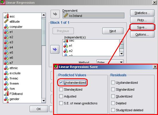
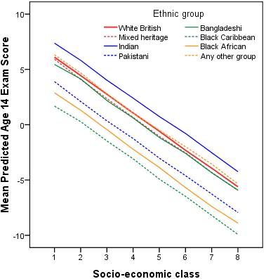
Add a tick in the ‘Predicted values (unstandardised)’ option in the pop-up box. This will create a new variable in your SPSS file called PRE_1 which will hold the predicted age 14 score for each student, as calculated by the model.

We can then plot these values to give us a visual display of the predicted variables. Let us look at the relationship between ethnic group and SEC. We will just plot the predicted values for boys since, as we have seen, the pattern of predicted values for girls will be identical except that every predicted value will be 1.234 points higher than the corresponding value for boys. We can plot the graph using the menu options as shown in the Foundation Module, or we can do this more simply using syntax: Creating a line graph for Age 14 achievement by ethnic group and SEC for boys only . The results are shown in Figure 3.8.1.

Figure 3.8.1: Regression lines for ethnic group, SEC and age 14 attainment

The important point you should notice is that the fitted regression lines for each ethnic group have different intercepts but the same slope, i.e. the regression lines are parallel. There are two equivalents ways of expressing the figure. We can say that the effect of SEC on attainment is the same for all ethnic groups, or we can say the effect of ethnicity on attainment is the same for all social classes. It’s the same thing (like two sides of a coin).

We will return to this type of line graph when we start to explore interaction effects on Page 3.11 but for now let’s discuss ways of refining our existing model further.

Navigation

Home
Modules
Site Guide
Module 3 Contents
Resources