-
- Mod 3 - Multiple Reg
- 3.1 Overview
- 3.2 The Model
- 3.3 Assumptions
- 3.4 Modelling LSYPE Data
- 3.5 Model 1: Ordinal Explanatory Variables
- 3.6 Model 2: Dichotomous Explanatory Variables
- 3.7 Model 3: Nominal Variables
- 3.8 Predicting Scores
- 3.9 Model 4: Refining the Model
- 3.10 Comparing Coefficients
- 3.11 Model 5: Interaction Effects 1
- 3.12 Model 6: Interaction Effects 2
- 3.13 Model 7: Value Added Model
- 3.14 Diagnostics and Assumptions
- 3.15 Reporting Results
- Quiz
- Exercise
- Mod 3 - Multiple Reg
Using Statistical Regression Methods in Education Research

3.7 Adding Nominal Variables with More than Two Categories (Model 3)
|
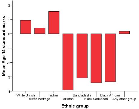
On Page 3.6 Figure 3.7.1: Bar chart of mean age 14 score by ethnic group
On Page 3.4 we mentioned the use of ‘dummy variables’ as a method for dealing with this issue. Where we have nominal variables with more than two categories we have to choose a reference (or comparison) category and then set up dummy variables which will contrast each remaining category against the reference category. See below for an explanation of how the ethnic group variable is coded into seven new dichotomous ‘dummy’ variables. Nominal variable with more than two categories: Ethnicity This requires the use of dummy variables. The variable is originally coded '0' to '7' with each code representing a different ethnic group. However we cannot treat this as an ordinal variable - we cannot say that 'Black Caribbean (coded '5') is 'more' of something than White British (coded '0'). What we need to do is compare each ethnic group against a reference category. The most sensible reference category is 'White British' (because it contains the largest number of participants), so we want to contrast each ethnic group against 'White British'. We do this by creating seven separate variables, one for each minority ethnic group (dummy variables). The group we leave out (White British) will be the reference group (‘0’ code). This has already been done in the dataset so why not take a look. The new variable 'e1' takes the value of '1' if the participant is of 'Mixed Heritage' and '0' otherwise, while 'e2' takes the value of '1' if the pupil is Indian and '0' otherwise, and so on.
We have already coded the dummy variables for you but it is important to know how it is done on SPSS. You can use the Transform > Recode into new variable route to create each new variable individually. We have discussed the use of Transform for creating new variables briefly in our Foundation Module The alternative to generating each dummy variable individually is using syntax. We have included the syntax for the recoding of the ethnicity variable below: Creating dummy variables for ethnicity
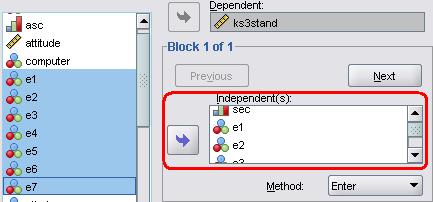
We can now include our dummy variables for ethnic group (e1 through to e7). Take the same familiar path through SPSS: Analyse > Regression > Linear. Add ks3stand as the Dependent and move all of the relevant variables into the Independents box: sec, gender, e1, e2, e3, e4, e5, e6 and e7.
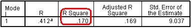
Click OK when you’re ready. You will see that the new model has improved the amount of variance explained with r2 = .170, or 17.0% of the variance (Figure 3.7.2), up from 15.5% in the previous model. We won’t print the ANOVA table again but it does show that the new model once again explains more variance than the baseline (mean) model to a statistically significant level. Figure 3.7.2: Model 3 summary
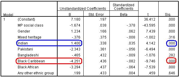
More interesting for our understanding and interpretation is the coefficients table (Figure 3.7.3). Figure 3.7.3: Regression coefficients for model 3
Firstly a quick glance at the b coefficients (Figure 3.7.3) shows SEC and gender are still significant predictors, with a decrease of -1.674 score points for every unit increase in SEC and with girls scoring 1.234 points higher than boys. The b-coefficients for the ethnic dummy variables can be interpreted in a similar way to the interpretation of gender. The coefficients represent the difference in age 14 test score between being in the specified category and being in the reference category (White British) when the other variables are all controlled. For example, the model indicates that Indian students achieve 1.40 more standard score points than White British students, while Black Caribbean student achieve -4.25 less standard score points than White British students. Remember these coefficient are after controlling for SEC and gender. Though it is clear that SEC score is the most important explanatory variable, looking down the t and sig columns tells us that actually most of the ethnic dummy variables make a statistically significant contribution to predicting age 14 score (p < .05). After we have controlled for SEC and gender, there is no statistically significant evidence that students of Mixed Heritage, Bangladeshi and Any Other ethnic group achieve different results to White British students. However on average Indian students score significantly higher than White British students while Pakistani, Black Caribbean and Black African pupils score significantly lower (p<.000). |