Checking the final version of the model

So far we have looked at building a multiple regression model in a very simple way. We have not yet engaged with the assumptions and issues which are so important to achieving valid and reliable results. In order to obtain the relevant diagnostic statistics you will need to run the analysis again, this time altering the various SPSS option menus along the way.

Let’s use this opportunity to build model 7 from the beginning. Take the following route through SPSS: Analyse> Regression > Linear and set up the regression. We will use model 7 which is: ks3stand as the outcome variable, with the explanatory variables as ks2stand, gender, e1-e7 (ethnicity) and sc0-sc7 (Socio-economic class). Don’t click ok yet!

We will need to make changes in the submenus in order to get access to the necessary information for checking the assumptions and issues. Let’s start with the Statistics and Plots submenus.

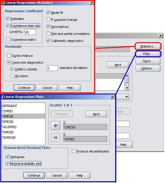
Many of these options should be familiar to you from the Simple Linear Regression Module.

We will request the Estimates, Descriptives and Model fit from the Statistics submenu. We also recommend that you get the Confidence Intervals this time as they provide the range of possible values for each of your explanatory variable’s regression (b) coefficients within which you can be 95% sure that the true value lies. In addition we now have the potential issue of our explanatory variables being too highly correlated, so we should also get hold of the Multicollinearity Diagnostics.

It is worth also collecting the Casewise Diagnostics. These will tell us which cases have residuals that are three or more standard deviations away from the mean. These are the cases with the largest errors and may well be outliers (note that you can change the number of standard deviations from 3 if you wish to be more or less conservative).

You should exercise the same options as before in the Plots menu. Create a scatterplot which plots the standardised predicted value (ZPRED) on the x-axis and the standardised residual on the y-axis (ZRESID) so that you can check the assumption of homoscedasticity. As before we should also request the Histogram and Normal Probability Plot (P-P plot) in order to check that our residuals are normally distributed. Head back to Page 2.7 of our previous module if you need to jog your memory about how to do all of this on SPSS.

We should also obtain some useful new variables from the Save menu.

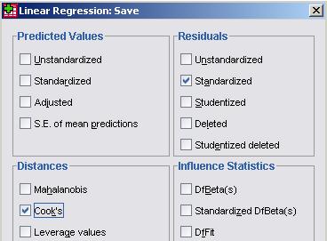
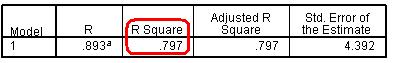
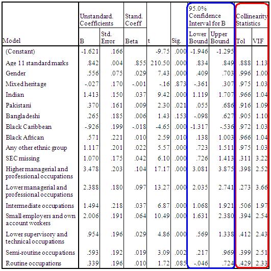
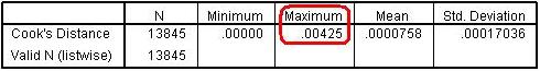
From the Residuals section it is worth requesting the Standardised residuals as these can be useful for additional analysis. It is also worth getting the Cook’s distance from the Distances section. The Cook’s distance statistic is a good way of identifying cases which may be having an undue influence on the overall model. Cases where the Cook’s distance is greater than 1 may be problematic. Once you have obtained them as a separate variable you can search for any cases which may be unduly influencing your model. We don’t need the Unstandardised Predicted values for our purposes here.

Now that we have selected our outcome and explanatory variables and altered all of the relevant submenus it is time to run the analysis... click OK.

SPSS seems to have had a great time and has spat out a vast array of tables and plots, some of which are so alarmingly large that they do not even fit on the screen! We hope that, by now, you are getting used to SPSS being overenthusiastic and do not find this too disconcerting! Rather than reproduce all of that extraneous information here we will discuss only the important bits.

The Descriptive Statistics table is always worth glancing over as it allows you to understand the basic spread of your data. Note that the dummy variables for ethnicity and SEC can only vary between 0 and 1. Next we have a truly monstrous Correlations table. We have not included it because it would probably crash the internet... or at least make this page harder to read! However, it is very useful to know the correlations between the variables and whether they are statistically significant. The Correlations table is also useful for looking for multicollinearity. If any two explanatory variables have a Pearson’s coefficient of 0.80 or greater there may be cause for concern – they may actually be measures of the same underlying factor. We have also ignored the Variables Entered/Removed table as it merely provides a summary of all of the variables we have included in our current model.

The model summary (Figure 3.14.1) provides us with a new value for r² for our expanded model, r² =.797. The model explains about 80% of the variance in age 14 score. From the ANOVA table we can see that F = 3198.072, df =17, p < .0005. This means that, as hoped, the regression model we have constructed is better at predicting the outcome variable than using the mean outcome (it generates a significantly smaller sum of residuals).

Figure 3.14.1: r and r² for final model

The Coefficients table (Figure 3.14.2) is frighteningly massive to account for the large number of variables it now encompasses. However, aside from a few small additions, it is interpreted in the exact same way as in the previous example so don’t let it see your fear! We won’t go through each variable in turn (we think you’re probably ready to have a go at interpreting this yourself now) but let’s look at the key points for diagnostics. Note we’ve had to shrink our table down to fit it on the screen!

Figure 3.14.2: Coefficients table for full model

Because we requested multicollinearity statistics and confidence intervals from SPSS you will notice that we have four more columns at the end of the coefficients table. The 95% confidence interval tells us the upper and lower bounds for which we can be confident that the true value of b coefficient lies. Examining this is a good way of ascertaining how much error there is in our model and therefore how confident we can be in the conclusions that we draw from it. Finally the Collinearity Statistics tell us the extent to which there is multicollinearity between our variables. If the value for the Tolerance is less than 10 and the value of the VIF is close to 1 for each explanatory variable then there is probably no cause for concern. The VIF for some of the SEC variables suggests we may have some issues with multicollinearity which require further investigation. However looking at the correlations table reveals that correlations between variables are weak despite often being statistically significant which allays our concerns about multicollinearity.

Collinearity Diagnostics emerge from our output next. We will not discuss this here because understanding the exact nature of this table is beyond the scope of this website. The table is part of the calculation of the collinearity statistics. The Casewise Diagnostics table is a list of all cases for which the residual’s size exceeds 3. We haven’t included it here because as you can see there are over 100 cases with residuals of this size! There are several ways of dealing with these outliers. If it looks as though they are the result of a mistake during data entry the case could be removed from analysis. Close to one hundred cases seems like a lot but is actually not too unexpected given the size of our sample – it is less than 1% of the total participants. The outliers will have a relatively small impact on the model but keeping them means our sample may better represent the diversity of the population.

We created a variable which provides us with the Cook’s Distance for each case which is labelled as COO_1 in your dataset. If a case has a Cook’s distance of greater than 1 it may be an overly influential case that warrants exclusion from the analysis. You can look at the descriptive statistics for Cook’s distance to ascertain if any cases are overly influential. If you have forgotten how to calculate the descriptive statistics, all you need to do is take the following route through SPSS: Analyze > Descriptive Statistics > Descriptives (see the Foundation Module if you require a reminder). Figure 3.14.3 shows the output. As you can see the maximum value of Cook’s distance in our sample is .00425 which far less than the value of 1 which may be a cause for concern. We do not appear to have any problematic cases in our sample.

Figure 3.14.3: Descriptive statistics for Cook’s distance Model 7

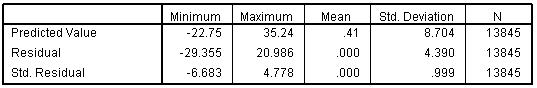
The Residuals Statistics (Figure 3.14.4) summarise the nature of the residuals and predicted values in the model (big surprise!). It is worth glancing at so you can get a better understanding of the spread of values that the model predicts and the range of error within the model.

Figure 3.14.4: Residual statistics for model

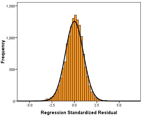
Next we have the plots and graphs that we requested. A Histogram of the residuals (Figure 2.14.5) suggests that they are close to being normally distributed but there are more residuals close to zero than perhaps you would expect.

Figure 3.14.5: Histogram of standardised model residuals

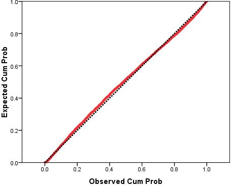
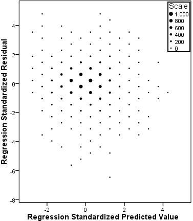
The P-P plot (Figure 3.14.6) is a little more reassuring. There does seem to be some deviation from normality between the observed cumulative probabilities of 0.2 and 0.6 but it appears to be minor. Overall there does not appear to be a severe problem with non-normality of residuals.

Figure 3.14.6: P-P plot of standardised model residuals

This Scatterplot (which we have altered with binning in Figure 3.14.7 to clarify) shows that the residuals are not distributed in any pattern with the predicted values. This suggests that our model does not violate the assumption of homoscedasticity.

Figure 3.14.7: Scatterplot of standardised residuals against standardised predicted values

Finally, we created a variable for the Standardised Residuals of the model which has appeared in your data file labelled as ZRE_1. If you wanted to perform certain analyses regarding which groups or cases the model is more accurate for (e.g. do certain ethnic groups have a smaller mean residual than others?) than creating this variable is very useful.

Now we have run our multiple linear regression with all of the explanatory variables let’s have a look at how to report the results...

Navigation

Home
Modules
Site Guide
Module 3 Contents
Resources