-
- Mod 3 - Multiple Reg
- 3.1 Overview
- 3.2 The Model
- 3.3 Assumptions
- 3.4 Modelling LSYPE Data
- 3.5 Model 1: Ordinal Explanatory Variables
- 3.6 Model 2: Dichotomous Explanatory Variables
- 3.7 Model 3: Nominal Variables
- 3.8 Predicting Scores
- 3.9 Model 4: Refining the Model
- 3.10 Comparing Coefficients
- 3.11 Model 5: Interaction Effects 1
- 3.12 Model 6: Interaction Effects 2
- 3.13 Model 7: Value Added Model
- 3.14 Diagnostics and Assumptions
- 3.15 Reporting Results
- Quiz
- Exercise
- Mod 3 - Multiple Reg
Using Statistical Regression Methods in Education Research

3.5 A Model with an Ordinal Explanatory Variable (Model 1)
|
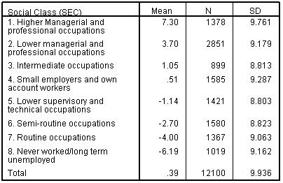
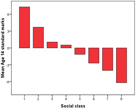
Rather than start by throwing all possible explanatory variables into the regression model let’s build it up in stages. This way we can get a feel for how adding different variables affects our model. Our outcome variable is ks3stand - the standard score in national tests taken at the end of Key Stage 3 (KS3) at age 14, which we used as the outcome measure in the previous module. To begin our analysis we will start with Social Economic Class (SEC) as a explanatory variable. SEC represents the socio-economic class of the home on a scale of '1' (Higher Managerial and professional occupations) to '8' (Never worked/long term unemployed). There is a strong relationship between SEC and mean age 14 score, as shown in Figures 3.5.1 and 3.5.2 below. Table 3.5.1: Mean age 14 score by SEC
Figure 3.5.2: Mean age 14 score by SEC
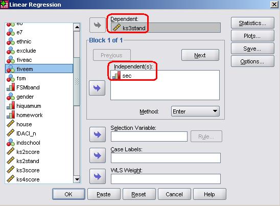
We will start by entering SEC in our regression equation. Take the following route through SPSS: Analyse> Regression > Linear. This is the exact same route which we took for simple linear regression so you may well recognise the pop-up window that appears. The variable ks3stand goes in the dependent box and the variable sec is placed in the independents box. Note that we have selected ‘Enter’ as our Method (see Page 3.2
We are not going to run through all of the diagnostic tests that we usually would this time – we will save that for when we add more variables over the coming pages! Let’s just click OK as it is and see what SPSS gives us.
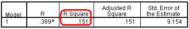
In this basic analysis SPSS has only provided us with four tables. The first simply tells us which variables we have included in the model so we haven’t reproduced that here. The other three provide more useful information about our model and the contribution of each of our explanatory variables. The process of interpreting most of these statistics is the same for multiple linear regression as we saw for simple linear regression in Module 2 Figure 3.5.3: Multiple r and r2 for model
The Model Summary (Figure 3.5.3) offers the multiple r and coefficient of determination (r2) for the regression model. As you can see r2 = .151 which indicates that 15.1% of the variance in age 14 standard score can be explained by our regression model. In other words the success of a student at age 14 is strongly related to the social economic class of the home in which they reside (as we saw in Figure 3.5.2). However there is still a lot of variation in outcomes between students that is not related to SEC. Figure 3.5.4: ANOVA for model fit
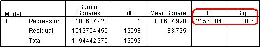
Whether or not our regression model explains a statistically significant proportion of the variance is ascertained from the ANOVA table (Figure 3.5.4), specifically the F-value (penultimate column) and the associated significance value. As before, our model predicts the outcome more accurately than if we were just using the mean to model the data (p < .000, or less than .0005, remembering that SPSS only rounds to 3 significant figures). Figure 3.5.5: Coefficients for model
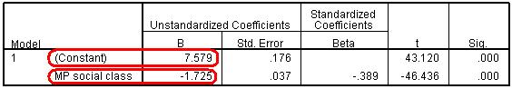
The Coefficients table (Figure 3.5.5) gives the Constant or intercept term and the regression coefficients (b) for each explanatory variable. The constant value (7.579) represents the intercept, which is the predicted age 14 score when SEC=0 (note that SEC is never actually 0 in our data where the values of SEC range from 1-8, the constant is just important for the construction of the model). The other value here is the regression coefficients (b) for SEC. This indicates that for every unit increase in SEC the model predicts a decrease of -1.725 in age 14 standard score. This may sound counter-intuitive but it actually isn’t – remember that SEC is coded such that lower values represent higher social class groups (e.g. 1 = ‘Higher Managerial and professional’, 8 = ‘Never worked/long term unemployed’). We can use the regression parameters to calculate the predicted values from our model, so the predicted age 14 score when SEC=1 (higher managerial) is 7.579 + (1*-1.725) = 5.85. By comparison the predicted age 14 score when SEC=8 (long term unemployed) is 7.579 + (8*-1.725) = -6.22. There is therefore roughly a 12 score point gap between the highest and lowest SEC categories, which is a substantial difference. Finally the t-tests and ‘sig.’ values in the last two rows tell us that the variable is making a statistically significant contribution to the predictive power of the model – it appears that SEC is since the t-statistic is statistically significant (p < .000). |