The key assumptions of multiple regression

The assumptions for multiple linear regression are largely the same as those for simple linear regression models, so we recommend that you revise them on Page 2.6. However there are a few new issues to think about and it is worth reiterating our assumptions for using multiple explanatory variables.

Linear relationship: The model is a roughly linear one. This is slightly different from simple linear regression as we have multiple explanatory variables. This time we want the outcome variable to have a roughly linear relationship with each of the explanatory variables, taking into account the other explanatory variables in the model.

Homoscedasticity: Ahhh, homoscedasticity - that word again (just rolls off the tongue doesn't it)! As for simple linear regression, this means that the variance of the residuals should be the same at each level of the explanatory variable/s. This can be tested for each separate explanatory variable, though it is more common just to check that the variance of the residuals is constant at all levels of the predicted outcome from the full model (i.e. the model including all the explanatory variables).

Independent errors: This means that residuals should be uncorrelated.

As with simple regression, the assumptions are the most important issues to consider but there are also other potential problems you should look out for:

Outliers/influential cases: As with simple linear regression, it is important to look out for cases which may have a disproportionate influence over your regression model.

Variance in all predictors: It is important that your explanatory variables... well, vary! Explanatory variables may be continuous, ordinal or nominal but each must have at least a small range of values even if there are only two categorical possibilities.

Multicollinearity: Multicollinearity exists when two or more of the explanatory variables are highly correlated. This is a problem as it can be hard to disentangle which of them best explains any shared variance with the outcome. It also suggests that the two variables may actually represent the same underlying factor.

Normally distributed residuals: The residuals should be normally distributed.

We’ve moved through these issues quite quickly as we have tackled most of them before. You can review the simple linear regression assumptions on Page 2.6 if you feel a little bit rusty.

Checking the assumptions

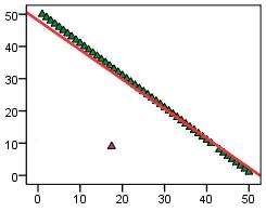
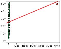
Here is an assumptions checklist for multiple regression:

1. Linear relationships, outliers/influential cases: This set of assumptions can be examined to a fairly satisfactory extent simply by plotting scatterplots of the relationship between each explanatory variable and the outcome variable. It is important that you check that each scatterplot is exhibiting a linear relationship between variables (perhaps adding a regression line to help you with this). Alternatively you can just check the scatterplot of the actual outcome variable against the predicted outcome.

Now that you're a bit more comfortable with regression and the term residual you may want to consider the difference between outliers and influential cases a bit further. Have a look at the two scatterplots below (Figures 3.3.1 & 3.3.2):

Figure 3.3.1: Scatterplot showing a simple outlier	Figure 3.3.2: Scatterplot showing an outlier that is an influential case

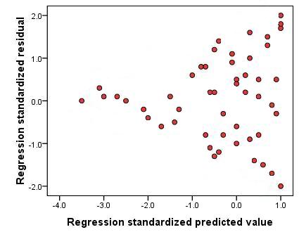
Note how the two problematic data points influence the regression line in differing ways. The simple outlier influences the line to a far lesser degree but will have a very large residual (distance to the regression line). SPSS can help you spot outliers by identifying cases with particularly large residuals. The influential case outlier dramatically alters the regression line but might be harder to spot as the residual is small - smaller than most of the other more representative points in fact! A case this extreme is very rare! As well as examining the scatterplot you can also use influence statistics (such as the Cook's distance statistic) to identify points that may unduly influence the model. We will talk about these statistics and how to interpret them during our example.

2. Variance in all explanatory variables: This one is fairly easy to check - just create a histogram for each variable to ensure that there is a range of values or that data is spread between multiple categories. This assumption is rarely violated if you have created good measures of the variables you are interested in.

3. Multicollinearity: The simplest way to ascertain whether or not your explanatory variables are highly correlated with each other is to examine a correlation matrix. If correlations are above .80 then you may have a problem. A more precise approach is to use the collinearity statistics that SPSS can provide. The Variance inflation factor (VIF) and tolerance statistic can tell you whether or not a given explanatory variable has a strong relationship with the other explanatory variables. Again, we'll show you how to obtain these statistics when we run through the example!

4. Homoscedasticity: We can check that residuals do not vary systematically with the predicted values by plotting the residuals against the values predicted by the regression model. Let's go into this in a little more depth than we did previously. We are looking for any evidence that residuals vary in a clear pattern. Let’s look at the examples below (Figure 3.3.3).

Figure 3.3.3: Scatterplot showing heteroscedasticity - assumption violated

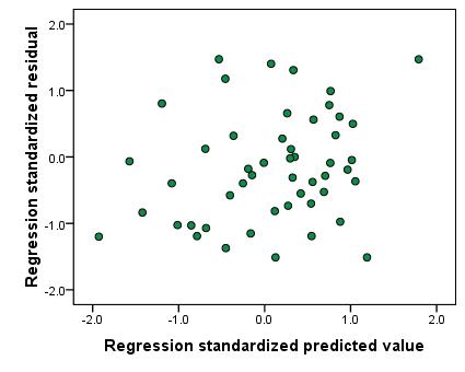
This scatterplot is an example of what a scatterplot might look like if the assumption of homoscedasticity is not met (this can be described as heteroscedasticity). The data points seem to funnel towards the negative end of the x-axis indicating that there is more variability in the residuals at higher predicted values than at lower predicted values. This is problematic as it suggests our model is more accurate when estimating lower values compared to higher values! In cases where the assumption of homoscedasticity is not met it may be possible to transform the outcome measure (see Extension A).

Figure 3.3.4: Scatterplot showing homoscedasticity - assumption met

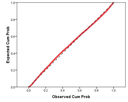
That's better! In Figure 3.3.4 the data points seem fairly randomly distributed with a fairly even spread of residuals at all predicted values.

5. Independent errors: As we have stated before this assumption is rather tricky to test but luckily it only really applies to data where repeated measures have been taken at several time points. It should be noted that, as we said on Page 2.6, if there is a high degree of clustering then multi-level multiple regression may be appropriate. Using the SPSS complex samples module, mixed module or separate multi-levelling modelling packages such as MLWin may be the only solution (see Page 2.6 for more detail).

6. Normally distributed residuals: A histogram of the residuals (errors) in our model can be used to check that they are normally distributed. However it is often hard to tell if the distribution is normal from just a histogram so additionally you should use a P-P plot as shown below (Figure 3.3.5):

Figure 3.3.5: P-P plot of standardised regression residual

As you can see the expected and observed cumulative probabilities, while not matching perfectly, are fairly similar. This suggests that the residuals are approximately normally distributed. In this example the assumption is not violated.

A note on sample size

The size of the data set that you're analysing can be very important to the regression model that you can build and the conclusions that you can draw from it. In order for your regression model to be reliable and capable of detecting certain effects and relationships you will need an appropriate sample size. There is a general rule of thumb for this:

This is useful BUT it should be noted that it is an oversimplification! A good sample size depends on the strength of the effect or relationship that you're trying to detect - the smaller the effect you’re looking for the larger the sample you will need to detect it! For example, you may need a relatively small sample to find a statistically significant relationship between age and reading ability. Reading ability usually develops with age and so you can expect a strong association will emerge even with a relatively small sample. However if you were looking for a relationship between reading ability and something more obscure, say time spent watching television, you would probably find a weaker correlation. To detect this weaker relationship and be confident that it exists in the actual population you will need a larger sample size.

On this website we're mainly dealing with a very large dataset of over 15,000 individual participants. Though in general it can be argued that you want as big a sample as practically possible some caution is required when interpreting data from large samples. A dataset this large is very likely to produce results which are 'statistically significant'. This is because the sheer size of the sample overwhelms the random effects of sampling - the more of the population we have spoken to the more confident we can feel that we have adequately represented them. This is of course a good thing but a 'statistically significant' finding can have the effect of causing researchers to overemphasise their findings. A p-value does not tell the researcher how large an effect is and it may be that the effect is statistically significant but so small that it is not important. For this reason it is important to look at the effect size (the strength) of an effect or relationship as well as whether or not it is statistically likely to have occurred by chance in a sample. Of course it is also important to consider who is in your sample. Does it represent the population you want it to?

If you would like more information about sample size we recommend that you check out Field (2009, p.645). There is also software that will allow you to estimate quite precisely the sample size you need to detect a difference of a given size with a given level of confidence. One example is the dramatically named ‘GPower’, which can be downloaded for free (the link is in our Resources). With this in mind let us put our new knowledge on regression analysis into practice by running through an example!

Navigation

Site Guide
Modules
Resources