-
- Mod 4 - Log Reg
- 4.1 Overview
- 4.2 Odds, Odds Ratios and Exponents
- Quiz A
- 4.3 A General Model
- 4.4 Log Reg Model
- 4.5 Logistic Equations
- 4.6 How good is the model?
- 4.7 Multiple Explanatory Variables
- 4.8 Methods of Log Reg
- 4.9 Assumptions
- 4.10 Example from LSYPE
- 4.11 Log Reg on SPSS
- 4.12 SPSS Log Reg Output
- 4.13 Interaction Effects
- 4.14 Model Diagnostics
- 4.15 Reporting the Results
- Quiz B
- Exercise
- Mod 4 - Log Reg
Using Statistical Regression Methods in Education Research

4.13 Evaluating Interaction Effects
|
We saw in Module 3 The first step is to add all the interaction terms, starting with the highest. With three explanatory variables there is the possibility of a 3-way interaction (ethnic * gender * SEC). If we include a higher order (3 way) interaction we must also include all the possible 2-way interactions that underlie it (and of course the main effects). There are three 2-way interactions: ethnic*gender, ethnic*SEC and Gender*SEC. Our strategy here is to start with the most complex 3-way interaction to see if it is significant. If it is not then we can eliminate it and just test the 2-way interactions. If any of these are not significant then we can eliminate them. In this way we can see if any interaction terms make a statistically significant contribution to the interpretation of the model. In this example we will use the MLR LSYPE 15,000
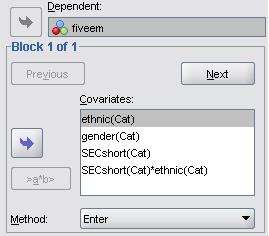
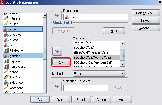
The masters of SPSS smile upon us, for adding interaction terms to a logistic regression model is remarkably easy in comparison to adding them to a multiple linear regression one! Circled in the image below is a button which is essentially the ‘interaction’ button and is marked as ‘>a*b>’. How very helpful! All you have to do is highlight the two (or more) variables you wish to create an interaction term for in the left hand window (hold down ‘control’ on your keyboard while selecting your variables to highlight more than one) and then use the ‘>a*b>’ button to move them across to the right hand window as an interaction term. The two variables will appear next to each other separated by a ‘*’. In this way you can add all the interaction terms to your model.
If we were to create interaction terms involving all levels of SEC we would probably become overwhelmed by the sheer number of variables in our model. For the two-way interaction between ethnicity and SEC alone we would have seven ethnic dummy variables multiplied by seven SEC dummy variables giving us a total of 49 interaction terms! Of course, we could simplify the model if we treated SEC as a continuous variable, we would then have only seven terms for the interaction between ethnic * SEC. While it would be a more parsimonious model (because it has fewer parameters to model the interaction), treating SEC as a continuous variable would mean omitting the nearly 3,000 cases where SEC was missing. The solution we have taken to this problem, as described before on Page 3.12 Even though we have chosen to use the three category SEC measure, the output is very extensive when we include all possible interaction terms. We have a total of 55 interaction terms (three for gender*SECshort, seven for ethnic*gender, 21 for ethnic*SECshort and a further 21 for ethnic*SECshort*gender). You will forgive us then if we do not ask you to run the analysis with all the interactions! Instead we will give you a brief summary of the preliminary analyses, before asking you to run a slightly less complex model. Our first model included all the three-way and two way interactions as well as the main effects. It established that three-way interaction was not significant (p=0.91) and so could be eliminated. Our second model then included just all the two-way interactions (and main effects). This showed that the gender*SECshort and the ethnic*gender interactions were also not significant but the ethnic*SECshort interaction was significant. The final model therefore eliminated all but the ethnic*SECshort interaction which needs to be included along with the main effects.
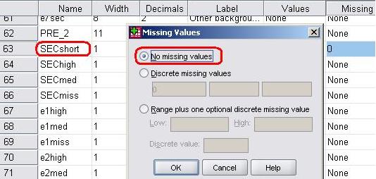
So let’s run this final model including the ethnic*SECshort interaction. Maybe you want to run through this example with us on SPSS (you can also follow it in our video demonstration Remember to tell SPSS which variables are categorical and set the options as we showed you on Page 4.11 Before running this model you will need to do one more thing. Wherever it was not possible to estimate the SEC of the household in which the student lived SECshort was coded 0. To exclude these cases from any analysis the ‘missing value’ indicator for SECshort is currently set to the value ‘0’. As discussed on Page 3.9
This will ensure that SPSS makes us a dummy variable for SEC missing. You can now click OK on the main menu screen to run the model!
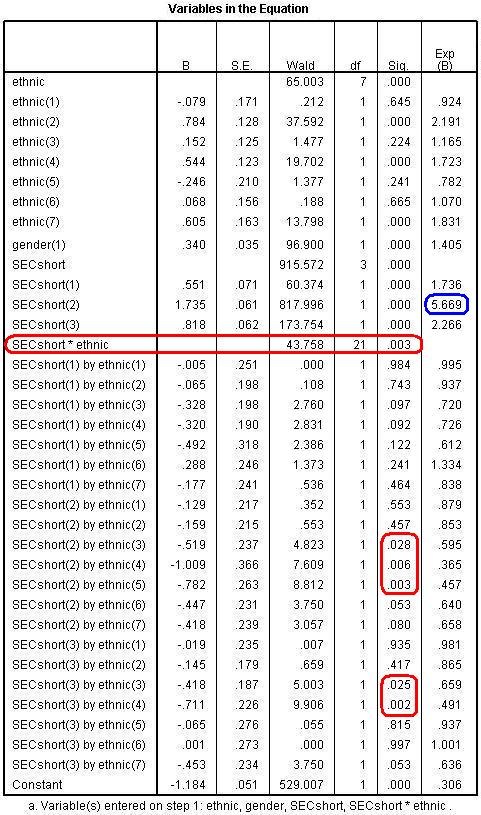
The results of this final model are shown below. Rather than show you all of the output as on the previous page (Page 4.12 Figure 4.13.1: Variables in the Equation Table with Interaction Terms
The overall Wald for the SECshort*ethnic interaction is significant (WALD=43.8, df=21, p<.005) so we proceed to look at the individual regression coefficients. You will need to refer to the Categorical Variables Encoding Table to remind yourself what each of these coefficients represents (for example SECshort(1)=missing; SECshort(2)= high SEC and SECshort(3)= middle SEC, with low SEC as the reference category). There are statistically significant coefficients for the interaction between Pakistani and middle and high SEC, between Bangladeshi and middle and high SEC and between Black Caribbean and high SEC. Working out the Odds Ratios (ORs) with interaction effects is somewhat tricky (remember we encountered a similar issue for multiple linear regression modules on Page 3.11
We can see that SEC has a substantial association with achievement among White British students. White British students from high SEC homes are 5.67 times more likely to achieve fiveem than White British students from low SEC homes. How do we determine the size of the SEC effect among other ethnic groups? Well, when interaction terms are included in the model we need to calculate the predicted probabilities by adding the B coefficients together, as we did in multiple linear regression. So to estimate the SEC gap for Black Caribbean students we add the coefficient for high SEC [SECshort(2)] and the B for the interaction between Black Caribbean and high SEC [SECshort(2) by ethnic(5)]. This gives = 1.735 + -.784 = 0.953. What does this mean? Not much yet – we need to take the exponent to turn it into a trusty odds ratio: Exp(0.953)=2.59 (we used the =EXP() function in EXCEL or you could use a calculator). This means that among Black Caribbean students High SEC students are only 2.6 times more likely to achieve fiveem than low SEC students - the SEC gap is much smaller than among White British students. The important point to remember is that you cannot simply add up the Exp(B)s to arrive here – it only works if you add the B coefficients in their original form and then take the exponent of this sum!
The model has told us what the ethnic gaps are among low SEC students (the reference category). Suppose I wanted to know what the estimated size of the ethic gaps was among high SEC students, how would I do this? To find out you would rerun the model but set high SEC as the base or reference category. The coefficients for each ethnic group would then represent the differences between the average for that ethnic group and White British students among those from high SEC homes. Currently SECshort is coded as follows with the last category used as the reference group.
We can simply recode the value for missing cases from 0 to 9 and set the reference category to the first value, so High SEC becomes the reference category, as shown below:
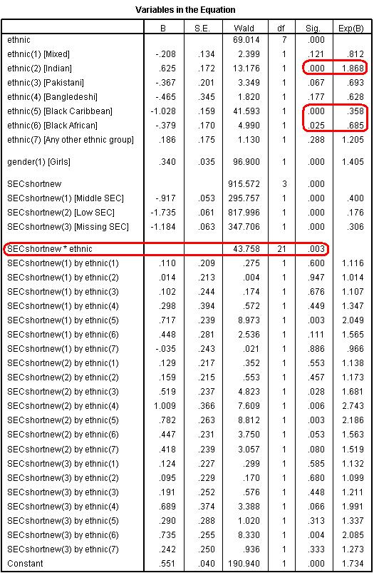
You can do this through the Transformation-Recode into new variable windows menu (see Foundation Module Syntax alert! RECODE SECshort (0=4) (ELSE=Copy) INTO SECshortnew. EXECUTE We then rerun the model simply adding SECshortnew as our SEC measure. It is important to note that computationally this is an exactly equivalent model to when low SEC was the reference category. The regression coefficients for other variables (for example, gender) are identical, the contrast between low and high SEC homes is the same (you can check the B value in the output below), and the R2 and log-likelihood are exactly the same. All that has varied is that the coefficients printed for ethnicity are now the contrasts among high SEC rather than low SEC homes. The output is shown below (Figure 4.13.2). For convenience we have added labels to the values so you can identify the groups. As you know, this is not done by SPSS so it is vital that you refer to the Categorical variables encoding table when interpreting your output. It is apparent that the ethnic gaps are substantially different among high SEC than among low SEC students. Among low SEC students the only significant contrasts were that Indian, Bangladeshi and Any other ethnic group had higher performance than White British (see Figure 4.13.1). However among students from high SEC homes while Indian students again achieve significantly better outcomes than White British students, both Black Caribbean (OR=.36, p<.005) and Black African (OR=.685, p<.025) are significantly less likely to achieve fiveem than White British students by a considerable margin. Black Caribbean students are only about one third as likely to achieve fiveem as White British high SEC students. In percentage terms we can say they are 64% (0.358-1 * 100) less likely to achieve fiveem than White British students of the same SEC group. Figure 4.13.2: Variables in the Equation Table with high SEC as the reference category If we wanted to evaluate the ethnic gaps among students from middle SEC homes we would simply follow the same logic as above, recoding our values so that middle SEC was the first (or last) category and setting the reference category appropriately.
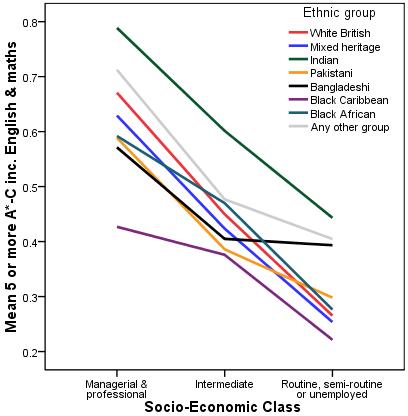
What is most helpful in understanding these interactions is to plot the data graphically. This gives us an easy visual indicator to help in interpreting the regression output and the nature of any interaction effects. We have done this in Figure 4.13.3 below. You can use Graphs > Legacy Dialogs > Line to create this graph or alternatively you can use the syntax below (see the Foundation Module Syntax Alert! GRAPH /LINE(MULTIPLE)=MEAN(fiveem) BY SECshort BY ethnic. Figure 4.13.3: Mean Number of Students with Five or More A*-C grades (inc. English and Maths) by SEC and Ethnicity
The line graph shows a clear interaction between SEC and ethnicity. If the two explanatory variables did not interact we would expect all of the lines to have approximately the same slope (for example, the lines on the graph would be parallel when there is no interaction effect) but it seems that the effect of SEC on fiveem is different for different ethnic groups. For example the relationship appears to be very linear for White British students (blue line) – as the socio-economic group becomes more affluent the probability of fiveem increases. This not the case for all of the ethnic groups. For example, with regard to Black Caribbean students there is a big increase in fiveem as we move from low SEC to intermediate SEC, but a much smaller increase as we move to high SEC. As you (hopefully) can see, the line graph is a good way of visualising an interaction between two explanatory variables. Now that we have seen how to create and interpret out logistic regression models both with and without interaction terms we must again turn our attention to the important business of checking that the assumptions underlying our model are met and that the results are not misleading due to any extreme cases. |
 ). In this model the ‘dependent’ variable is fiveem (our