-
- Mod 4 - Log Reg
- 4.1 Overview
- 4.2 Odds, Odds Ratios and Exponents
- Quiz A
- 4.3 A General Model
- 4.4 Log Reg Model
- 4.5 Logistic Equations
- 4.6 How good is the model?
- 4.7 Multiple Explanatory Variables
- 4.8 Methods of Log Reg
- 4.9 Assumptions
- 4.10 Example from LSYPE
- 4.11 Log Reg on SPSS
- 4.12 SPSS Log Reg Output
- 4.13 Interaction Effects
- 4.14 Model Diagnostics
- 4.15 Reporting the Results
- Quiz B
- Exercise
- Mod 4 - Log Reg
Using Statistical Regression Methods in Education Research

4.4 The Logistic Regression Model
|
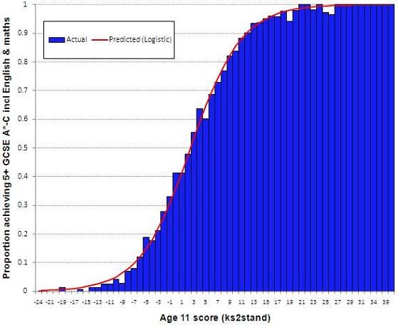
To see this alternative form for the relationship between age 11 score and fiveem, let us plot the actual data from LSYPE. In Figure 4.4.1 the blue bars show the actual proportion of students with each age 11 test score that achieved fiveem. Figure 4.4.1: Probability of 5+ GCSE A*-C including English & maths by age 11 test score We can see that the relationship between age 11 score and fiveem actually takes the form of an S shaped curve (a ‘sigmoid’). In fact whenever we have a binary outcome (and are thus interested in modelling proportions) the sigmoid or S shaped curve is a better function than a linear relationship. Remember that in linear regression a one unit increase in X is assumed to have the same impact on Y wherever it occurs in the distribution of X. However the S shape curve represents a nonlinear relationship between X and Y. While the relationship is approximately linear between probabilities of 0.2 and 0.8, the curve levels off as it approaches the ceiling of 1 and the floor of 0. The effect of a unit change in age 11 score on the predicted probability is relatively small near the floor and near the ceiling compared to the middle. Thus a change of 2 or 3 points in age 11 score has quite a substantial impact on the probability of achieving fiveem around the middle of the distribution, but much larger changes in age 11 score are needed to effect the same change in predicted probabilities at the extremes. Conceptually the S-shaped curve makes better sense than the straight line and is far better at dealing with probabilities.
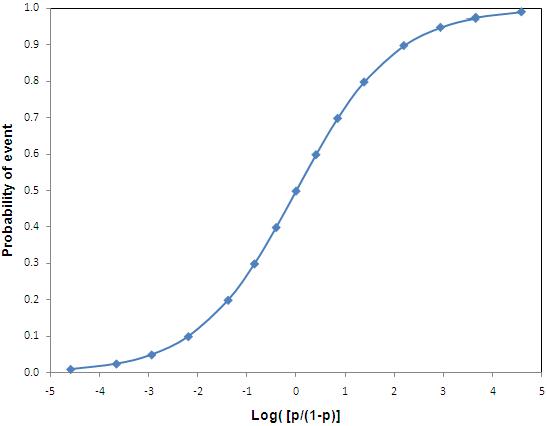
There are many ways to generate an S shaped curve mathematically, but the logistic function is the most popular and easiest to interpret. A function is simply a process which transforms data in a systematic way – in this example it transforms log odds into a proportion. We described on Page 4.2 Log [p/(1-p)] = a + bx. The logistic function transforms the log odds to express them as predicted probabilities. First, it applies the reverse of the log (called the exponential or anti-logarithm) to both sides of the equation, eliminating the log on the left hand side, so the odds can be expressed as: p/(1-p) = Exp(a+bx). Second, the formula can be rearranged by simple algebra to solve for the value p. p = Exp(a+bx) / [ 1 + Exp(a+bx)] Note: You will have to take our word on this, but a formula p / (1-p) =x can be rearranged to p = x / (1+x). So the logistic function transforms the log odds into predicted probabilities. Figure 4.4.2 shows the relationship between the log odds (or logit) of an event occurring and the probabilities of the event as created by the logistic function. This function gives the distinct S shaped curve. Figure 4.4.2: The logistic function Look back to Figure 4.4.1 where the blue bars shows the actual proportion of students achieving fiveem for each age 11 test score. We have superimposed over the actual figures a red line that shows the predicted probabilities of achieving fiveem as modelled from a logistic regression using age 11 test score as the explanatory variable. Comparing these predicted probabilities (red line) to the actual probability of achieving fiveem (blue bars) we can see that the modelled probabilities fit the actual data extremely well.
The log odds are more appropriate to model than probabilities because log odds do not have the floor of 0 and the ceiling of 1 inherent in probabilities. Remember the probability of an event occurring cannot be <0 or >1. What the log odds does is to ‘stretch’ the proportion scale to eliminate these floor and ceiling effects. They do this by (i) transforming the probabilities to odds, and (ii) taking the log of the odds.
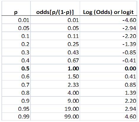
Odds remove the ceiling We saw in Figure 4.4.1 that there is a non-linear relationship between X and Y - for example, we need larger changes in X to effect the same proportionate increase in Y at the ceiling compared to near the middle. Odds can model this property because larger changes in odds are needed to effect the same change in the probabilities when we are at the ceiling than at the middle of the curve. Let’s look at specific figures using Figure 4.4.3 which shows the relationship between probabilities, odds and log odds. Figure 4.4.3: Probabilities, odds and log odds
A change in the probability of an event occurring from .5 to .6 is associated with a change in odds from 1.0 to 1.5 (an increase of 0.5 in the odds). However a similar change in probability from .8 to .9 reflects a much larger change in the odds from 4.0 to 9.0 (an increase of 5 in the odds). Thus modelling the odds reflects the fact that we need larger changes in X to effect increases in proportions near the ceiling of the curve than we do at the middle.
Log odds remove the floor (as well as the ceiling) Transforming probabilities into odds has eliminated the ceiling of 1 inherent in probabilities, but we are still left with the floor effect at 0, since odds, just like proportions, can never be less than zero. However taking the log of the odds also removes this floor effect.
The log odds still has the non-linear relationship with probability at the ceiling, since a change in p from .5 to .6 is associated with an increase in log odds from 0 to 0.4, while a change in probability from .8 to .9 is associated with an increase in log odds from 1.39 to 2.20 (or 0.8). However they also reflect the non-linear relationship at the floor, since a decrease in probability from .5 to .4 is associated with an decrease in log odds from 0 to -0.4, while a decrease in probability from .2 to .1 is associated with an decrease in log odds from -1.39 to -2.20 (or -0.8) (see Figure 4.4.3). Also, as we discussed on Page 4.2 |