-
- Mod 4 - Log Reg
- 4.1 Overview
- 4.2 Odds, Odds Ratios and Exponents
- Quiz A
- 4.3 A General Model
- 4.4 Log Reg Model
- 4.5 Logistic Equations
- 4.6 How good is the model?
- 4.7 Multiple Explanatory Variables
- 4.8 Methods of Log Reg
- 4.9 Assumptions
- 4.10 Example from LSYPE
- 4.11 Log Reg on SPSS
- 4.12 SPSS Log Reg Output
- 4.13 Interaction Effects
- 4.14 Model Diagnostics
- 4.15 Reporting the Results
- Quiz B
- Exercise
- Mod 4 - Log Reg
Using Statistical Regression Methods in Education Research

4.3 A General Model for Binary Outcomes
|
The example we have been using until now is very simple because there is only one explanatory variable (gender) and it has only two levels (0=boys, 1=girls). With this in mind, why should we calculate the logistic regression equation when we could find out exactly the same information directly from the cross-tabulation? The value of the logistic regression equation becomes apparent when we have multiple levels in an explanatory variable or indeed multiple explanatory variables. In logistic regression we are not limited to simple dichotomous independent variables (like gender) we can also include ordinal variables (like socio-economic class) and continuous variables (like age 11 test score). So the logistic regression model lets us extend our analysis to include multiple explanatory variables of different types.
We can think of the data in Figure 4.2.1 (Page 4.2
As another way to consider the logic of logistic regression, consistent with what we have already described but coming at it from a different perspective, let’s consider first why we cannot model a binary outcome using the linear regression methods we covered in modules 2 and 3. We will see that significant problems arise in trying to use linear regression with binary outcomes, which is why logistic regression is needed.
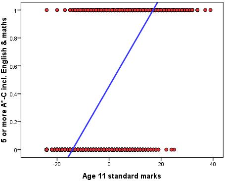
A new example: Five or more GCSE passes at A*-C including English and maths For this example let us take as our outcome as whether a student achieves the conventional measure of exam success in England, which is achieving five or more GCSE passes at grades A*-C, including English and maths (fiveem). This is a frequently used measure of a student’s ‘success’ in educational achievement at age 16. It is also used at an institutional level in school performance tables in England by reporting the proportion of students in each secondary school achieving this threshold, attracting considerable media attention. Our variable fiveem is coded ‘0’ if the student did not achieve this threshold and ‘1’ if the student did achieve it. We want to predict the probability of achieving this outcome depending on test score at age 11. We can fit a linear regression to this binary outcome as shown in Figure 4.3.1 below.
Figure 4.3.1: A linear regression of age 11 test score against achieving five or more GCSE grades A*-C including English and maths (fiveem)
The linear regression of age 11 score on fiveem give the following regression equation: Ŷ = .454 + .032 * X (where X=age 11 score which can range from -24 to 39).
The predicted values take the form of proportions or probabilities. Thus at the average age 11 score (which was set to 0, see Extension A
However there are two problems with linear regression that make it inappropriate to use with binary outcomes. One problem is conceptual and the other statistical.
Lets deal with the statistical problem first. The problem is that a binary outcome violates the assumption of normality and homoscedasticity inherent in linear regression. Remember that linear regression assumes that most of the observed values of the outcome variable will fall close to those predicted by the linear regression equation and will have an approximately normal distribution (See Page 2.6
The second problem is conceptual. Probabilities and proportions are different from continuous outcomes because they are bounded by a minimum of 0 and a maximum of 1, and by definition probabilities and proportions cannot exceed these limits. Yet the linear regression line can extend upwards beyond 1 for large values of X and downwards below 0 for small values of X. Look again at Figure 4.3.1. We see that students with an age 11 score below -15 are actually predicted to have a less than zero (<0) probability of achieving fiveem. Equally problematic are those with an age 11 score above 18 who are predicted to have a probability of achieving fiveem greater than one (>1). These values simply make no sense.
We could attempt a solution to the boundary problem by assuming that any predicted values of Y>1 should be truncated to the maximum of 1. The regression line would be straight to the value of 1, but any increase in X above this point would have no influence on the predicted outcome. Similarly any predicted values of Y<0 could be truncated to 0 so any decrease in X below this point would have no influence on the predicted outcome. However there is another functional form of the relationship between X and a binary Y that makes more theoretical sense than this ‘truncated’ linearity. Stay tuned… |