Non-normally distributed data

There are occasions where your continuous variables may not be normally distributed. This is often caused by ceiling or floor effects where data points gather at the extremes of the scale but it can occur for a great many reasons. This can lead to many a researcher tantrum – after all, doesn’t this mean that regression analysis cannot be used? In actual fact this is not always the case as sometimes non-normal data can be sensibly ‘transformed’. 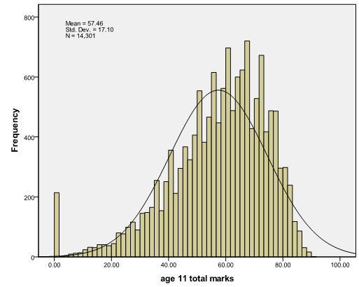For an example let’s plot a histogram of age 11 exam scores (KS2score), complete with a superimposed normal curve (Figure A1). If you like, you can follow us through this process using the LSYPE 15,000 data set: Graphs > Legacy Dialogs > Histograms. When you get the pop-up menu, move the variable ks2score into the Variable box – you can also Display normal curve simply by putting a tick in the relevant box. Click OK when you’re ready.

Figure A1: Histogram of KS2 score

Let’s take a close look at our histogram. Two things are notable about the distribution:

• There is a floor effect - a large number of cases with an average age 11 mark of zero. These are not missing cases - students who were absent from the ks2 tests have already been excluded and in the SPSS data file they have the system missing value (indicated as ‘.’). The scores of zero indicate the 214 students whose attainment is judged by their teachers to be so low that they are working at a level below that assessed by the tests. These represent about 1.5% of the students in the sample. We do not want to exclude these students as we have a genuine measure of their attainment; it is just that we are not able to differentiate between them (all we can say is that they all got the lowest possible score). While they do not fit well into a normal distribution it would be a quite an omission to exclude them from the analysis.
• Second, the distribution does not fit the normal curve very well! The data are skewed and there is a long tail of lower scores. Technically the distribution would be described as negatively skewed, as there are more data points than expected in the left tail of the distribution. (If there were more data points than expected in the right tail of the distribution it would be described as positively skewed).

This non-normal distribution is a significant problem if we want to use parametric statistical tests with our data, since these methods assume normally distributed continuous variables. What can we do about this? Luckily SPSS has a number of options to transform scores in situations where the distribution is not normal.

Transforming to normal scores

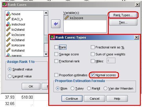
In this section we will transform our ks2 score to the normal equivalent. From the menu you would do this as follows: Transform -> Rank. You will get the window shown below. Click on Rank types and you will get another pop-up box where you should check the box marked Normal scores. The other options do not need to be altered so just click Continue and then OK on the main window...

 

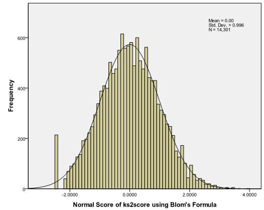
This creates a new variable prefixed by N to indicate normalised, so here the new variable is called NkS2scor. Let’s plot a histogram of Nks2scor to examine its distribution (use the same SPSS commands as before, just swap the variable):

Figure A2: Histogram of the transformed variable (Nks2scor)

Compare Figure A2 with Figure A1. See how much it has changed? We now have a distribution that is very close to the normal distribution. In essence the transformation has ranked the scores, calculated the proportion of cases at each rank, and applied the Z score that equates to that proportion based on the normal distribution (e.g. cases at the 50^th percentile will have a score of 0, cases at the 84^th percentile a score of 1, cases at the 95^th percentile a score of 1.64 etc). It is not important to know exactly how this transformation is calculated, but something called the BLOM formula calculates the proportions. There is still the peak at the bottom of the distribution representing those students who were performing below the level assessed by the tests, but we will live with this for the reasons described earlier – these individuals constitute an important group and excluding them would bias our findings.

The KS2 Standard Score

This new variable has a mean of 0 and standard deviation of 1. However for the purposes of our examples it will be easier to work with larger numbers without decimal places, so we will just multiply Nks2scor by 10 and round the figures up to create a new variable called ks2stand (the Key Stage 2 standard mark). You already have this in your dataset so don’t worry too much about adding these additional changes!

Other Transformations

There are a range of other transformations that can be used to correct non-normal data distributions. While many students are (understandably) suspicious of such transformations (it sounds like fudging or fixing your data!) the key principle is that you apply the same transformation to all your data points. We don’t intend to go through all the transformations here, but a good transformation should be a relatively simple and straightforward operation. For example a square root transformation is often use when the outcome data (for example income) might be positively skewed (for example by having a small number of very high salaries for millionaires). Taking the square root of large values has more of an impact than taking the square root of small values. Consequently taking the square root of your data points will bring any large scores closer to the centre. Other common transformations include taking the log [log(x)] or the reciprocal [1/x] of your data. See Field, 2009 (p153-164) for a detailed discussion of transformation of data.

How to complete a normal score transformation

...However, if you want to learn more about computing variables here is a brief guide to how we did it. Transform > Compute Variable will open up the Compute pop-up menu.

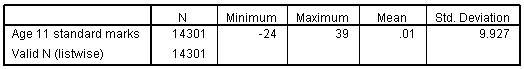
We need to type the name of our new variable into the small window in the top left called Target Variable. We have called it ks2stand2 for the purposes of this demonstration because we already have the ks2stand2 variable saved! Our aim is to multiply the variable by 10 and round it to the nearest full number. From the Function group window on the far right select Arithmetic and then Rnd(1) from the Functions and Special Variables window just below it. RND(?) will appear in the Numeric Expression window at the top. The long window on the left contains all of our variables – pull the newly created Nks2score in to the expression (it will replace the question mark). To multiply it by 10 simply use the numeric pad in the middle of the pop-up menu (or the one on your keyboard) to add ‘*10’. Finally we need to complete the expression by telling SPSS how many decimal places we want our score rounded to. Simply place a coma followed by ‘1’ to tell SPSS we want the nearest whole number (if we wanted 1 decimal place we would put 0.1, two decimal places 0.01, etc.). Once you are happy with your expression click OK to create the new variable!

SYNTAX ALERT!!!

If you can cope with a bit of computer language this can be done with much more haste and much less hassle by using the following syntax:
COMPUTE kS2stand=RND(nks2scor*10,1) 

The descriptive statistics for ks2stand are shown below (Figure A3). The mean score is still 0 but the standard deviation is now 10, and the scores range from -24 to 39. The previous histogram (Figure A2) below shows the distribution of scores.

Figure A3: Descriptive statistics for ks2 standardised score

Exercise

We have followed the same process as described above to create transformed variables for age 14 standard score (ks3stand) and age 16 standard score (ks4stand). You will find these in the data file. As an optional exercise follow the example above to transform ks3score to the normal score equivalent. Does your transformed variable have the same distribution as the variable ks3stand in the file? Check your answer here!

Navigation

Home
Modules
Site Guide
Module 2 Contents
Resources