Using Statistical Regression Methods in Education Research

1.4 SPSS: An Introduction
|
This section will provide a brief orientation of the SPSS software. Don’t worry; we’re not going to try to replicate the user manual - just run you through the basics of what the different windows and options are. Note that you may find that the version of SPSS you are using differs slightly from the one we use here (we are using Version 17). However the basic principles should be the same though things may look a little different. The best way to learn how to use software is to play with it. SPSS may be less fun to play with than a games console but it is more useful! Probably... If you would like a more in depth introduction to the program we refer you to Chapter 3 of Field (2009) or the Economic and Social Data Service (ESDS) guide to SPSS. Both of these are referenced in our Resources There are two main types of window, which you will usually find open together on your computer’s task bar (along the bottom of the screen). These windows are the Data Editor and the Output Viewer.
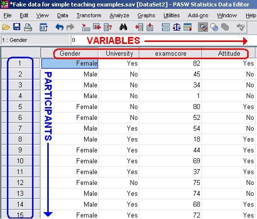
The data editor is a spreadsheet in which you enter your data and your variables. It is split in to two windows: Data View and Variable View. You can swap between them using the tabs in the bottom left of the Data Editor. Data View: Each row represents one case (unit) in your sample (this is usually one participant but it could be one school or any other single case). Each column represents a separate variable. Each case’s value on each variable is entered in the corresponding cell. So it is just like any 2 x 2 (row by column) spreadsheet!
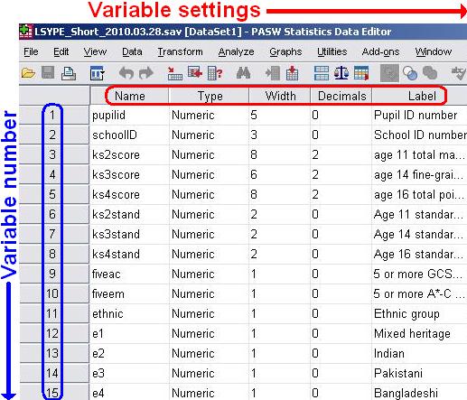
Variable View: This view allows you to alter the settings of your variables with each row representing one variable. Across the columns are different settings which you can alter for each variable by going to the corresponding cell. These settings are characteristics of the variable. You can add labels, alter the definition
of
the level of measurement of the data (e.g. nominal, ordinal, scale) and assign numeric values to nominal or ordinal responses (more on this in Page 1.7
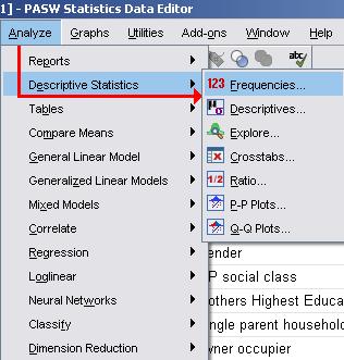
The lists of options at the top of the screen provide menus for managing, manipulating, graphing, and analysing your data. The two most frequently used are probably Graphs and Analyze. They open up cascading menus like the one below:
Analyze is the key for performing regression analyses as well as for gaining descriptive statistics, tabulating data, and exploring associations between variables. The Graphs menu allows you to draw the various plots, graphs and charts necessary to explore and visualise your data. When you are performing analyses or producing other types of output on SPSS you will often open a pop-up menu to allow you to specify the details. We will explore the available options when we come to discuss individual tasks but it is worth noting a few general features.
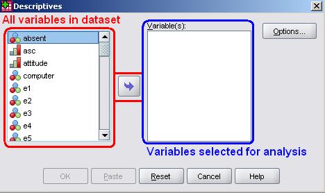
On the left of the pop-up window you will see a list of all the variables in your dataset. You will usually be required to move the variables you are interested in across to the relevant empty box or boxes on the right. You can either drag and drop the variable or highlight it and then move it across with the arrow:
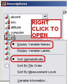
You will become very familiar with these arrows and the menu windows in general the more you use SPSS! On the far right there are usually buttons which allow you to open further submenus and tinker with the settings for your analysis (e.g. Options, as above). The buttons at the bottom of the window perform more general functions such as accessing the Help menu, starting again or correcting mistakes (Reset or Cancel) or, most importantly, running the analysis (OK). Of course this description is rather general but it does give you a rough indication of what you will encounter. It is useful to note that you can alter the order that your list of available variables appear in along with whether you see just the variable names or the full labels by right clicking within the window and selecting from the list of options that appears (see below). This is a useful way of finding and keeping track of your variables! We recommend choosing ‘Display Variable Names’ and ‘Sort Alphabetically’ as these options make it easier to see and find your variables.
On the main screen there are also a number of buttons (icons) which you can click on to help you keep track of things. For example, you can use the pair of snazzy Find binoculars to search through your data for particular values (you can do this with a focus on individual variables by clicking on the desired column). The labelbutton allows you to switch between viewing the numerical values for each variable category and the text label that the value represents (for ordinal and nominal variables). You can also use the select cases button if you want to examine only specific units within your sample.
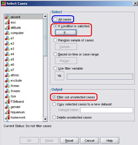
Clicking on the Select Cases button (or accessing it through the menus, Data > Select Cases) opens up the following menu:
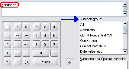
This menu allows you to select specific cases for you to run analysis on. Most of the time you will simply have the All cases option selected as you will want to examine the data from all of your participants. However, on occasion it may be that you only want to look at a certain sub-sample of your data (all of the girls for example), in this case the If option will come into play (more on this soon!). In addition you can select a sub-sample completely at random (Random sample of cases) or select groups based on the order in which they are arranged in the data set (Based on time or case range). These last two options are rarely used but they are worth knowing about. It is also important to note that you have a number of options regarding how to deal with your selection of cases (your sub-sample). The Output options allow you to choose what happens to the cases that you select. The default option ‘Filter out unselected cases’ is best – all this does is temporary exclude unselected cases, placing a line through them in the data editor. They are not deleted - you can reintroduce them again through the select cases menu at any time. ‘Copy selected cases to a new dataset’ can be useful if you will be working with a specific selection in detail and want to store them as a separate dataset. Your selected cases will be copied over to a new data editor window which you can save separately. Finally the option to ‘Delete unselected cases’ is rather risky – it permanently removes all cases you did not select from the dataset. It could be useful if you have a huge number of cases that needs trimming down to a manageable quantity but exercise caution and have backup files of the original unaltered dataset. If, like us, you tend to make mistakes and/or change your mind frequently then we recommend you avoid using this option all together! The most commonly used selection option is the Ifmenu so let’s take a closer look at it. To be honest the If menu (shown in part below) terrifies us! This is mainly because of the scientific calculator keypad and the vast array of arithmetic functions that are available on the right. The range of options available is truly
mind-blowing! We
will not even attempt to explain all of these options to you as most of them rarely come into use. However we have highlighted our example in the image. Most uses of the If menu really will be this simple. Girls are coded as ‘1’ in the LSYPE dataset. If we wish to select only girls for our analyses we need to tell SPSS to select a case only if the gender variable has a value of ‘1’. So in order to select only girls we simply put ‘gender =1’ in the main input box and click Continue to return to the main Select Cases menu. This is a simple example but the principles are simple. We only briefly describe these functions here but you can calculate almost any ‘if’ situation using this menu. It is worth exploring the possibilities yourself to see how the ‘If’ menu can best serve you! This calculator like setup will also appear in the Compute option which we discuss later (Page 1.7), so we are coming back to it if you are confused. Once back at the main Select Cases menu simply click OK to confirm your settings and SPSS will do the rest. Remember to change it back when you are ready to look at the whole sample again!
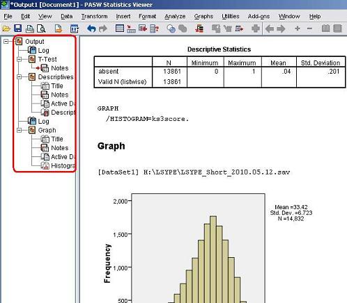
The output viewer is where all of the statistics, charts, tables and graphs that you request will pop into existence. It is a scary place to the uninitiated... Screen spanning ‘pivot tables’ which are full of numbers rounded to three decimal places. Densely packed scatterplots which appear to convey nothing but chaos. Sentences that are written in a bizarre computer language that appear to make absolutely no sense whatsoever (For example: ‘DESCRIPTIVES VARIABLES = absent STATISTICS = MEAN STDDEV MIN MAX’... yes SPSS, whatever you say – actually we come to learn about this so-called ‘Syntax on Page 1.7 Trust us when we say that those who withstand the initial barrage of confusion will grow to appreciate the output viewer... it brings forth the detailed results of your analysis which greatly informs your research! The trick is learning to filter out the information that is not important. With regard to regression analysis (and a few other things!) this website will help you to do this. Below is an example of what the output viewer looks like.
Tables and graphs are displayed under their headings in the larger portion of the screen on the right. On the left (highlighted) is an output tree which allows you to jump quickly to different parts of your analysis and to close or delete certain elements to make the output easier to read. SPSS also records a log in the output viewer after each action to remind you of the analyses you have performed and any changes you make to the dataset. One very useful feature of the output is how easy it is to manipulate and export to a word processor. If you double-click on a table or graph an editor window opens which gives you access to a range of options, from altering key elements of the output to making aesthetic changes. These edited graphs/tables can easily be copied and pasted into other programs.
There is nothing better at grabbing your reader’s attention than presenting your findings in a well-designed graph! We will show you how to perform a few useful tricks with these editors on Page 1.5 Let us now move on to talk a little bit more making graphs. |