Types of Research Design

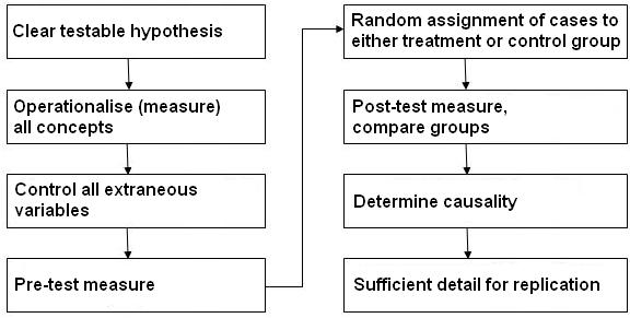
This website does not aim to provide an in depth discussion about research methods as there are comprehensive alternative sources available if you want to learn more about this (check out our Resources page, particularly Cohen, Manion & Morrison, 2007; 6^th Edition; chapters 6-13). However, it is worth discussing a few basics. In general there are two main types of quantitative research design.

Experimental designs: Experimental designs are highly regarded in many disciplines and are related to experiments in the natural sciences (you know the type - where you nearly lose your eyebrows due to some confusion about whether to add the green chemical or the blue one). The emphasis is on scientific control, making sure that all the variables are held constant with the exception of the ones you are altering (independent variable) and the ones you are measuring as outcomes (dependent variable). Figure 1.3.1 illustrates the type of process you may take:

Figure 1.3.1: The process of experimental research

A Quasi-experiment is one where truly random assignment of cases to intervention or to control groups is not possible. For example, if you wanted to examine the impact of being a smoker on performance in a Physical Education exam you could not randomly assign individuals into ‘smoking’ and ‘non-smoking’ groups – that would not be ethical (or possible!). However you could recruit individuals who are already smokers to your experimental group. You could control for factors like age, SEC, gender, marital status (anything you think might be important to your outcome) by matching your ‘smoking’ participants with similar ‘non-smoking’ participants. This way you compare two groups that were matched on key variables but differed with regard to your independent variable – whether or not they smoke. This is imperfect as there may be other factors (confounding variables) that differ between the groups but it does allow you to use a form of experimental design in a natural context. This type of approach is more common in the social sciences where ethical and practical concerns make random allocation of individuals problematic.

Non-experimental designs: These designs gather substantial amounts of data in naturally occurring circumstances, without any experimental manipulation taking place. At one level the research can be purely descriptive (e.g. what is the relationship between ethnicity and student attainment?). However with careful selection and collection of data and appropriate analytic methods, such designs allow the use of statistical control to go beyond a purely descriptive approach (e.g. can the relationship between ethnicity and attainment be explained by differences in socio-economic disadvantage?). By looking at relationships between the different variables it can be possible for the researcher to draw strong conclusions that generalise to the wider population, although conclusions about causal relationships will be more speculative than for experimental designs.

For example, secondary schools differ in the ability of their students on intake at age 11 and this impacts very strongly on the pupils attainment in national exams at age 16. As a result ‘raw’ differences in exam results at age 16 may say little about the effectiveness of the teaching in a given school. You can’t directly compare grammar schools to secondary modern schools because they accept students from very different baseline levels of academic ability. However if you control for pupils’ attainment at intake at age 11 you can get a better measure of the school’s effect on the progressof pupils. You can also use this type of statistical control on other variables that you feel are important such as socio-economic class (SEC), ethnicity, gender, time spent on homework, attitude to school, etc. All of this can be done without the need for any experimental manipulation. This type of approach and the statistical techniques that underlie it are the focus of this website.

 

Quantitative/Qualitative methods or Quantitative/Qualitative data?

In some ways we don’t really like to use the term ‘quantitative methods’ as it somehow suggests that they are totally divorced from ‘qualitative methods’. It is important to avoid confusing methods with data. As Figure 1.3.2 suggests, it is more accurate to use the terms ‘quantitative’ and ‘qualitative’ to describe data rather than methods, since any method can generate both quantitative and qualitative data.

Figure 1.3.2: Research methods using different types of data

Quantitative data	Method	Qualitative data
Highly structured questions	Interviews	Loose script or guide
Closed questions	Questionnaire	Open-ended questions
Detailed coding schemes	Observation	Participant observation
Content analysis	Documents	Impressions & inferences
Standardised test score	Assessment	Formative judgement

You may be conducting face-to-face interviews with young people in their own homes (as is the case in the dataset we are going to use throughout these modules) but choose a highly structured format using closed questions to generate quantitative data because you are striving for comparable data across a very large sample (15,000 students as we shall see later!). Alternatively you may be interested in a deep contextualised account from half a dozen key individuals, in which case quantitative data would be unlikely to provide the necessary depth and context. Selecting the data needed to answer your research questions is the important thing, not selecting any specific method.

 

Operational measures

The hallmark of quantitative research is measurement - we want to measure our key concepts and express them in numerical form. Some data we gather as researchers in education are directly observable (biological characteristics, the number of students in a class etc.), but most concepts are unobservable or ‘latent variables’. For any internal mental state (anxiety, motivation, satisfaction) or inferred characteristic (e.g. educational achievement, socio-economic class, school ethos, effective teachers etc) we have to operationalise the concept, which means we need to create observable measures of the latent construct. Hence the use of attitude scales, checklists, personality inventories, standardised tests and examination results and so on. Establishing the reliability and validity of your measures is central but beyond the scope of this module. We refer you to Muijs (2004) for a simple introduction and any general methods text (e.g. Cohen et. al., 2007, Newby, 2009) for further detail.

 

Variables and values

The construct we have collected data on is usually called the variable (e.g. gender, IQ score). Particular numbers called values are assigned to describe each variable. For example, for the variable of IQ score the values may range from 60-140. For the variable gender the values may be 0 to represent ‘boy’ and 1 to represent ‘girl’, essentially assigning a numeric value for each category. Don’t worry, you’ll get used to this language as we go through the module!

 

Levels of measurement

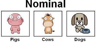
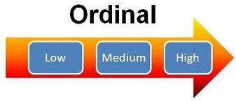
As we have said, the hallmark of quantitative research is measurement, but not every measurement is equally precise: saying someone is ‘tall’ is not the same as saying someone is 2.0 metres. Figure 1.3.3 shows us that quantitative data can come in three main forms: continuous, ordinal and nominal.

Figure 1.3.3: Levels of quantitative measurement 

Apologies for the slightly childish cartoon animals, we just liked them! Particularly the pig - he looks rather alarmed! Perhaps somebody is trying to make him learn something horrible... like regression analysis. Nominal data is of a categorical form with cases being sorted into discrete groups. These groups are also mutually exclusive; each case has to be placed in one group only. Though numbers are attached to these categories for analysis the numbers themselves are just labels - they simply represent the name of the category. Ethnicity is a good example of a nominal variable. We may use numbers to identify different ethnic groups (e.g. 0= White British, 1= mixed heritage, 2=Indian, 3=Pakistani etc) but the numbers just represent or stand for group membership, ‘3’ does not mean Pakistani students are three times more of ethnicity than White British students!

Ordinal datais also of a categorical form in which cases are sorted into discrete groups. However, unlike nominal data, these categories can be placed into a meaningful order. Social economic class is a good example of this. Different social economic groups are ranked based on how relatively affluent they are but we do not have a precise measure of how different each category is from one another. Though we can say people from the ‘higher managerial’ group are better off than those from the ‘routine occupations’ group we do not have a measure of the size of this gap. The differences between each category may vary.

Continuous data (scale) is of a form where there is a wide range of possible values which can produce a relatively precise measure. All the points on the scale should be separated by the same value so we can ascertain exactly how different two cases are from one another. Height is a good example of this. Somebody who is 190cm tall is 10cm taller than somebody who is 180cm tall. It is the exact same difference as between someone who is 145cm tall and someone who is 155cm tall. This may sound obvious (actually that part is obvious!) but although collecting data which is continuous is desirable surprisingly few variables are quantified in such a powerful manner! Test score is a good example of a scale variable in education.

All of these levels of data can be quantified and used in statistical analysis but must usually be treated slightly differently. It is important to learn what these terms mean now so that they do not return to trip you up later! Field (2009), pages 7-10 discusses the types of data further (see the Resources page).

Navigation

Home
Modules
Site Guide
Module 1 Contents
Resources