Using Statistical Regression Methods in Education Research

1.9 Probability and Inferential Stats
|
We discussed populations and sampling on Page 1.2
Inferential statistics are used to make generalisations about the characteristics of your sample, or associations between variables in your sample, to the characteristics/associations in the wider population. Such inferences require you to have a suitably large and representative sample. They also require you to make certain assumptions about your data, many of which can be directly tested. Usually when you are conducting research you wish to test a hunch or a hypothesis that you have about a population. There are several steps for testing your hypothesis:
Let’s start by talking about hypotheses. You probably noticed that there are two types of hypothesis mentioned in these steps; your initial hypothesis (often called the alternate hypothesis) and something called the null hypothesis. In order to explain these, let us take an example of a specific research question: Do girls have higher educational achievement than boys at age 14? Fortunately a measure of educational achievement at age 14 is available through national tests in English, mathematics and science which can be used to create a continuous (scale) outcome variable. We can use a particular statistical test called an independent t-test (see Page 1.10
In essence the process of hypothesis testing works like the UK legal system; you assume that the effect or relationship you are looking for does not exist, unless you can find sufficient evidence that it does… Innocent until proven guilty! We test to see if there is a difference between the mean scores for boys and girls in our sample and whether it is sufficiently large to be true of the population (remembering to take into account our sample size). Imagine we find a difference in the age 14 test scores of boys and girls in our sample such that boys have, on average, lower scores than girls. This could be a fair representation of the wider population or it could be due to chance factors like sampling variation. There is a chance, however small, that we inadvertently selected only the boys with low attainment so our sample does not represent the whole population fairly. The independent t-test, like many statistical analyses, lets us compute a test of statistical significance to find out how likely it is that any difference in scores resulted just from sampling variation. To understand this properly you will need to be introduced to the p-value...
A p-value is a probability. It is usually expressed as a proportion which can also be easily interpreted as a percentage:
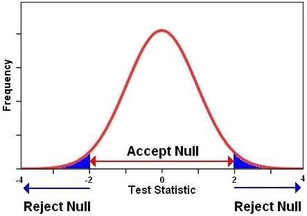
P-values become important when we are looking to ascertain how confident we can be in accepting or rejecting our hypotheses. Because we only have data from a sample of individual cases and not the entire population we can never be absolutely (100%) sure that the alternative hypothesis is true. However, by using the properties of the normal distribution we can compute the probability that the result we observed in our sample could have occurred by chance. To clarify, we can calculate the probability that the effect or relationship we observe in our sample (e.g. the difference between boys and girls mean age 14 test score) could have occurred through sampling variation and in fact does not exist in the population as a whole. The strength of the effect (the size of the difference between the mean scores for boys and girls), the amount of variation in scores (indicated by the standard deviation) and the sample size are all important in making the decision (we will discuss this in detail when we report completing independent t-tests on Page 1.10 Conventionally, where there is less than a 5% probability that the results from our sample are due to chance the outcome is considered statistically significant. Another way of saying this is that we are 95% confident there is a ‘real’ difference in our population. This is our confidence level. You are therefore looking for a p-value that is less than .05, commonly written as p <.05. Results significant at the 1% level (p<.01), or even the 0.1% level (p<.001), are often called "highly" significant and if you want to be more sure of your conclusions you can set your confidence level at these lower values. It is important to remember these are somewhat arbitrary conventions - the most appropriate confidence level will depend on the context of your study (see more on this below). The way that the p-value is calculated varies subtlety between different statistical tests, which each generate a test statistic (called, for example, t, F or X2 depending on the particular test). This test statistic is derived from your data and compared against a known distribution (commonly a normal distribution) to see how likely it is to have arisen by chance. If the probability of attaining the value of the test statistic by chance is less than 5% (p<.05) we typically conclude that the result is statistically significant. Figure 1.9.1 shows the normal distribution and the blue ‘tails’ represent the standardized values (where the mean is 0 and the standard deviation is 1) which allow you to reject the null hypothesis. Compare this to Figure 1.8.3 on Page 1.8 Figure 1.9.1: Choosing when to Accept and When to Reject the Null Hypothesis In other words, if the probability of the result occurring by chance is p<.05 we can conclude that there is sufficient evidence to reject the null hypothesis at the .05 level. There is only a 5% or 1 in 20 likelihood of a difference of this size arising in our sample by chance, so is likely to reflect a ‘real’ difference in the population. Note that either way we can never be absolutely certain, these are probabilities. There is always a possibility we will make one of two types of error:
The balance of the consequences of these different types or error determines the level of confidence you might want to accept. For example if you are testing the efficacy of a new and very expensive drug (or one with lots of unwanted side effects) you might want to be very confident that it worked before you made it widely available, you might select a very stringent confidence level (e.g. p<.001) to minimize the risk of a false positive (type I) error. On the other hand if you are piloting a new approach to teaching statistics to students you might be happy with a lower confidence level (say p<.05) to determine whether it is worth investigating the approach further. Before leaving p-values we should note that the p-value tells us nothing about the size of the effect. In large samples even very small differences may be statistically significant (bigger sample sizes increase the statistical power of the test). See Page 1.10
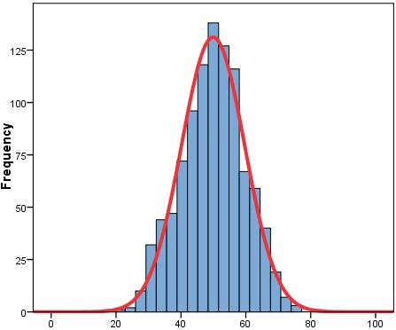
A core issue in generalising from our sample to the wider population is establishing how well our sample data fits to the population from which it came. If we took lots of random samples from our population, each of the same number of cases, and calculated the mean score for each sample, then the sample means themselves would vary slightly just by chance. Suppose we take 10 random samples, each composed of 10 students, from the Year 11 group in a large secondary school and calculate the mean exam score for each sample. It is probable that the sample means will vary slightly just by chance (sampling variation). While some sample means might be exactly at the population mean, it is probable that most will be either somewhat higher or somewhat lower than the population mean. So these 10 sample means would themselves have a distribution with a mean and a standard deviation (we call this the 'sampling distribution'). If lots of samples are drawn and the mean score calculated for each, the distribution of the means could be plotted as a histogram (like in Figure 1.9.2). Figure 1.9.2: Histogram of mean scores from a large number of samples
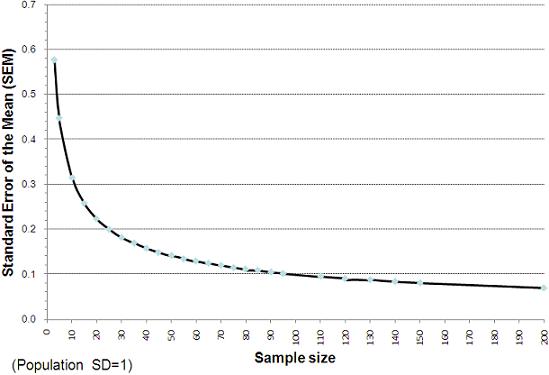
The standard deviation of the distribution of the sample means is called the standard error (SE). The SE is extremely important in determining how confident we can be about the accuracy of the sample mean as a representation of the population mean. Suppose Figure 1.9.2 was the result of drawing many random samples, each composed of 10 cases, from a population where the mean score was 50. The standard deviation of the distribution of the sample means (the standard error) is approximately 10 score points. We can use the properties of the normal distribution to calculate the range above or below the population mean within which we would expect any given sample mean to lie (given our sample size). Two-thirds (68%) of the sample means would lie between +/- 1 SE of the population mean and 95% of samples means would lie within +/- 2 SE of the population mean. For the example in Figure 1.9.2 we can say that 68% of the means (from random samples of 10 cases) would lie between 40 and 60, and 95% of the means (from random samples of 10 cases) would lie between 30 and 70. These ‘confidence intervals’ are very useful and will crop up frequently (in fact we say more about their uses below). Crucially the SE will vary depending on the size of the samples. With larger samples we are more likely to get sample mean scores that cluster closely around the population mean, with smaller samples there is likely to be much more variability in the sample means. Thus the greater the number of cases in the samples the smaller the SE. Figure 1.9.3 shows the relationship between sample size and the SE. Figure 1.9.3: Relationship between standard error of the mean (SEM) and sample size
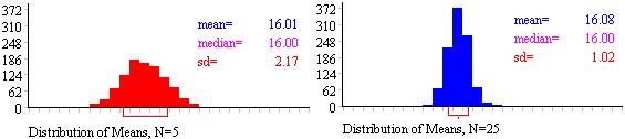
We understand that taking the ‘mean of the means’ and all that this entails may be a fairly complicated idea so we thought you might like to use this online toy which allows you to model sampling distributions Figure 1.9.4: Influence of sample size on SE Note: the value labelled SD in the figure is actually the standard error, because it is the SD of the distribution of means from several samples. Note that the means of the two sampling distributions are very similar. With a sufficient number of samples the mean of the sampling distribution will be centred at the same value as the population mean. However look at the SE. You can see how the SE shrinks when the larger sample size is used. In the first case, when each sample is composed of just 5 cases (N=5) the SE is 2.17. For the second case (where each sample has 25 observations, N=25) the SE is much smaller (1.02). This means the range of values within which 95% of sample means will fall is much more tightly clustered around the population mean. In practice of course we usually only have one sample rather than several: we do not typically have the resources to collect hundreds of separate samples. However we can estimate the SE of the mean quite well from knowledge of the SD and size of our sample according to the simple formula: It turns out that as samples get large (usually defined as 30 cases or more) the sampling distribution has a normal distrubution which can be estimated quite well from the above formula. You will notice this chimes with Figure 1.9.3. The reduction in the SE as we increase our sample size up to 30 cases is substantial while the incremental reduction in the SE by increasing our sample sizes beyond this is much smaller. This is why you will often see advice in statistical text books that a minimum sample size of 30 is advisable in many research contexts.
Let’s take a practical look at confidence intervals. An error bar plot can be drawn to help you visualize confidence intervals. Let’s use the LSYPE dataset (LSYPE 15,000
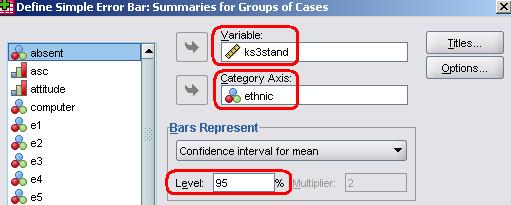
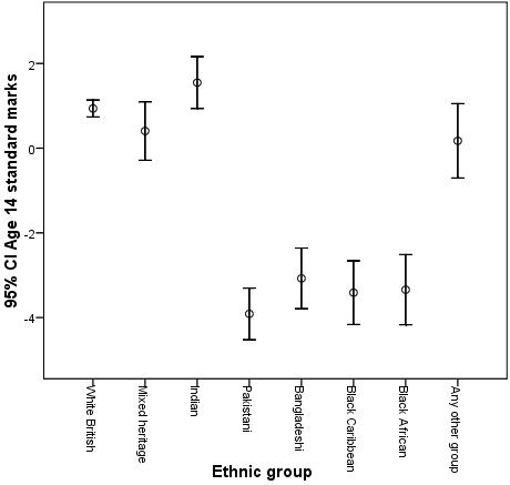
We will move age 14 test score (ks3score) into the Variable box and ethnic onto the Category Axis. Note the section titled Bars Represent which allows you to define the confidence interval – the default of 95% is the most commonly used, so we’ll stick to that, but it is useful to know it can be altered to match the context. Click OK when you are happy with the settings and Figure 1.9.5 should appear. Figure 1.9.5: Mean age 14 score by ethnicity with 95% Confidence intervals
The circle in the middle of each line represents the mean score for that ethnic group. The extension of the line represents the range in which we are 95% confident that the ‘true’ mean lies for the group (+/- 2 SE). Note how the confidence interval for White British students is comparatively narrower than the intervals for the other ethnic groups. This is because the sample size for this group is much larger than for the other groups (see Figure 1.5.1, Page 1.5 We can see from these error bars that, even though there are differences in the mean scores of the Pakistani, Bangladeshi, Black African and Black Caribbean groups, their confidence intervals overlap, meaning that there is insufficient evidence to suggest that the true population means for these groups differ significantly. However, such overlap in confidence intervals does not occur when we compare, for example, the White British students with these ethnic groups. The White British students score more highly at age 14 on average and the confidence intervals do not overlap. Overall the error bar plot suggests that on average White British, Mixed Heritage and Indian groups achieve a significantly higher age 14 test score than the Pakistani, Bangladeshi, Black African and Black Caribbean groups. We have shown you some of the basics of probability and started to consider how to analyse differences between group means. Let’s now expand on this and show you some of the different methods of comparing means using SPSS. |