Requesting a model with interaction terms

First ask for an ordinal regression through selecting Analyse>Regression>Ordinal as we did on Page 5.6. To specify interaction terms in SPSS ordinal we use the ‘Location’ submenu, so click on the ‘Location’ button. What we want to do now is specify not a ‘Main Effects’ but a ‘Custom’ model, so place a tick in the ‘Custom’ button as shown in the image below.

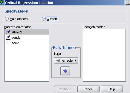
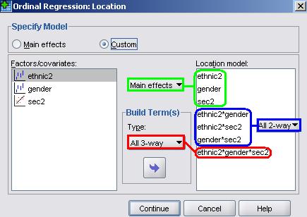
We now need to build our model. The logic of the approach to testing interactions is as we have described earlier in Module 3 (linear regression) and Module 4 (logistic regression). We start by specifying a full model that includes all the main effects, plus all 2-way interactions plus the three-way interaction. We then run this model and if the highest order interaction (here the 3-way interaction between ethnic2 * Sec2 * gender) is not significant it can be removed. We then run the model with the main effects and all the 2-way interactions, again subsequently eliminating any non-significant 2-way interaction terms.

To build this full model we hold down the CTRL key and click on ethnic2, gender and Sec2 in the ‘Factors/covariates’ box so all three variables are highlighted, then in the ‘Build terms’ box click ‘main effects’, and then drag (or click on the arrow) to move these to the ‘Location model’ box. Then do the same but click on ‘All 2-way’ in the ‘build terms’ box, and lastly again with ‘All 3-way’ in the build terms box as shown below:

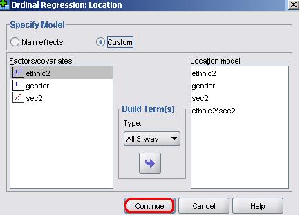
We have decided not to bombard you with the output but running this analysis on the data indicated no statistically significant 3-way interaction so this term was removed. Running a subsequent model with all 2-way interactions revealed no significant 2-way interactions between ethnic2*gender or Sec2*gender but a highly significant ethnic2*Sec2 interaction. Rather than repeating this analysis here, we will just request the model including the main effects and the significant ethnic2*sec2 interaction. You can remove the ethnic*gender*sec, gender*sec2 and ethnic2*gender terms by clicking on them and dragging (or using the reverse arrow) to move them back to the Factors/covariates box, leaving just the main effects and the ethnic2*sec2 interaction in the Location model. This is what the final version of the Location submenu will look like:

Click ‘Continue’ and then OK to run the model.

Interpreting the results with interactions

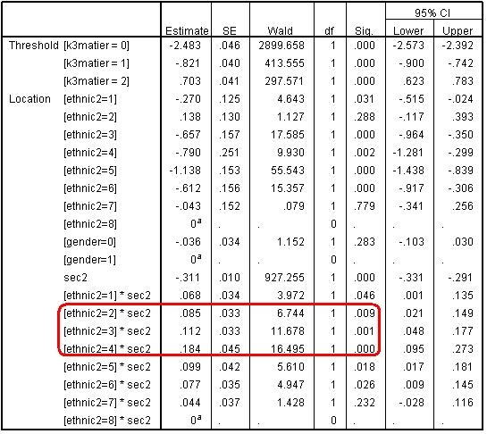
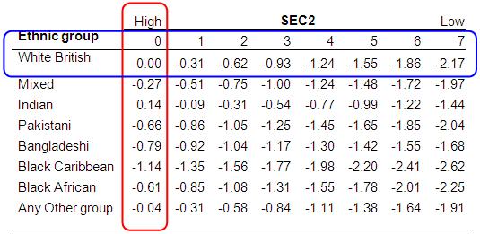
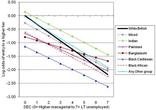
Examining the linear part of the model (the logits)

The parameter estimates are shown below (Figure 5.7.1). We can see that the interaction terms are all highly significant, particularly so for Indian, Pakistani and Bangladeshi students.

Figure 5.7.1: Parameter Estimates for Model with Interaction Terms

The significant interaction terms indicates the slope of the assumed linear relationship between SEC and entry to a higher tier varies significantly between ethnic groups. Just as we did when looking at interactions on Page 3.11 and Page 4.13 we can understand the interaction best by calculating the predicted values for each ethnic group by SEC combination and plotting these graphically. If we work with the linear part of the model (the logits) this will most clearly display the form of the interaction.

Just as with linear regression, we can think of the line representing the relationship between SEC and the predicted logit for entry to higher tiers as having the formula:

Y= a + b₁x₁ + b₂x₂ + b₃x₃ ...etc.

Because the effect of gender is a constant (it does not interact significantly with either ethnic2 or Sec2) then we only need to be concerned with three parameters: a= the intercept (the coefficients for ethnic group when Sec2=0); b₁x₁ representing the coefficient and value respectively for Sec2, and b₂x₂ represents the coefficient and values respectively for each of the ethnic2*Sec2 interactions.

The intercepts are just the ethnic group coefficients when Sec2=0. Because White British are the reference group for ethnicity their logit is represented by zero and the coefficients for each ethnic group are contrasts against White British. These values can be read directly from the SPSS output and are highlighted in red on Figure 5.7.2.

We then need to calculate the change in the logit for different levels of Sec2. The printed value of Sec2 in the SPSS output (-.311) is the unit change in logits associated with a one unit increase in the value of Sec2 for the reference group, i.e. White British students. So to calculate the predicted logits at each level of Sec2 for White British students we simply multiply -.311 by the respective value of Sec2. So for White British students from SEC=5 (semi-routine homes) the predicted logit is: 0 + (-.311 * 5) = -1.55. These predicted values are highlighted by the blue box on Figure 5.7.2.

For ethnic minority students the slope for Sec2 is moderated by the ethnic2*sec2 interaction. For example for Black Caribbean students from SEC=5 (semi-routine homes) the predicted logit is: -1.14 + (-.311 * 5) + (.099 * 5) = -2.20. It gives exactly the same result, but is slightly computational easier, to calculate the unit change in logits for each unit change in SEC for Black Caribbean (-.311 + .099 = -.211). We can then just multiply -.211 by the respective values of Sec2 and do this for all levels of Sec2. 

We follow the same process as above for each minority ethnic group. These predicted values are shown in the rest of Figure 5.7.2. We have used EXCEL to calculate the predicted logits shown in Figure 5.7.2 and to plot the relationship graphically Figure 5.7.3.

Figure 5.7.2: Predicted logits for each ethnic group and SEC combination from the ethnic2*sec2 interaction model

Figure 5.7.3: Predicted logits for each ethnic group and SEC combination from the ethnic2*sec2 interaction model

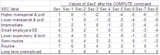
Examining the ORs

The above figure shows the relationship in terms of log odds (logits). What does this mean in terms of ORs? The OR for each ethnic group when sec2=0 (higher managerial and professional occupations) can be found directly by exponentiating the ethnic coefficients. For example the OR for Black Caribbean students is exp(-1.138)= 0.32, so for Black Caribbean students from homes in the highest SEC category the odds of being entered for a higher tier are only one third (0.32) the odds for White British students, or conversely the odds for White British students from the highest SEC category being entered for a higher tier are over three times (1/.32=3.12) the odds for Black Caribbean student being entered.

What about the ethnic group ORs at other levels of SEC? Exponentiating the values in the body of Figure 5.7.2 will give the ORs for each SEC and ethnic combination relative to the overall reference group (White British students from higher managerial & professional homes). This is fine, but what we really want are the ORs that compare each minority group to their White British peers within each SEC category.

The easiest way to calculate the ethnic group ORs at different values of SEC is simply to RECODE SEC to a new variable (Sec2) where the zero value represents the reference category of interest. This means the coefficients (and the associated standard errors and p values) for each ethnic group will give the contrast with White British students for the reference SEC category. This can easily be done by using the COMPUTE command to recode the original SEC variable. For example we used the following syntax to create the new variable sec2 taking one away from the value of SEC for each case.

We also adjusted the ‘Missing’ setting in the Variable View such that ‘-1’ (and not 0) was the missing value. This gives Sec2 the values we have used in the above analysis where higher managerial and professional homes is the reference category (0). You can see the recoded values for sec2 in the column labelled ‘Sec-1’ of Figure 5.7.4 below.

Figure 5.7.4: Varying the reference category for SEC using the COMPUTE command

Suppose we want long term unemployed to be the reference category for SEC. We can do this by subtracting 8 from every value of SEC to create a temporary SEC variable (SECtemp). This is the SPSS syntax:

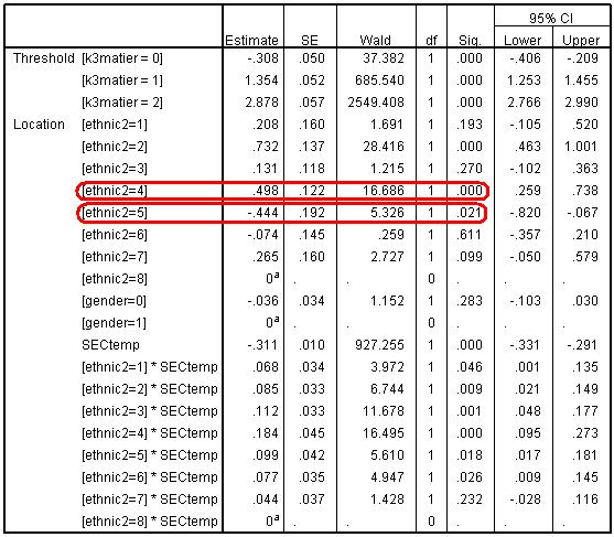
This gives SECtemp the values in the last column of Figure 5.7.4 labelled ‘Sec-8’. Now long term unemployed are the reference (0) category. If you run the regression again with this new coding of SEC (remembering to change the ‘Missing’ setting to ‘-9’ and the ‘measure’ column to ordinal) you will get the regression output shown below (Figure 5.7.5).

Figure 5.7.5: Parameter estimates with long term unemployed as the reference group

Now the coefficients (and standard errors and p values) for each ethnic group represent the contrasts when the SEC reference category is long term unemployed. As you would expect, these are substantially different for some ethnic groups from the ORs among students from higher managerial & professional homes. For example among the lowest SEC homes Bangladeshi pupils are significantly more likely than White British pupils to be entered for higher tiers (OR= exp(.498)= 1.65, p<.005). Black Caribbean students are still less likely than White British to be entered for a higher tier (OR = exp(-.444) = 0.64, p<.02), but this is a smaller degree of under-representation than we saw among students from the highest SEC homes where the OR was 0.32.

Evaluating model fit

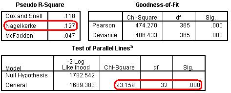
The interactions of ethnic2*sec2 are highly statistically significant, and, as we can see from Figure 5.7.6, including them has increased the Nagelkerke R² from 12.4% to 12.7%. However the goodness-of-fit test still indicates a less than adequate fit, and the test of parallel lines still formally rejects the proportional odds assumption. We therefore need to consider further refinements to our model.

Figure 5.7.6: Statistics for Evaluating the Model

Navigation

Home
Modules
Site Guide
Module 5 Contents
Resources