So let’s see how to complete an ordinal regression in SPSS, using our example of NC English levels as the outcome and looking at gender as an explanatory variable.

Data preparation

Before we get started, a couple of quick notes on how the SPSS ordinal regression procedure works with the data, because it differs from logistic regression. First, for the dependent (outcome) variable, SPSS actually models the probability of achieving each level or below (rather than each level or above). This differs from our example above and what we do for logistic regression. However this makes little practical difference to the calculation, we just have to be careful how we interpret the direction of the resulting coefficients for our explanatory variables. Don’t worry; this will be clear in the example. Second, for categorical (nominal or ordinal) explanatory variables, unlike logistic regression, we do not have the option to directly specify the reference category (LAST or FIRST, see Page 4.11) as SPSS ordinal automatically takes the LAST category as the reference category. So for our gender variable (scored boys=0, girls=1) girls will be the reference category and the coefficients will be for boys. Again this is not a huge problem because if we want to we can simply RECODE our variables to force a particular category as the reference category (e.g. if we wanted boys to be the reference category we could recode gender so girls=0 and boys=1). It is, however, slightly fiddly and annoying!

Requesting an ordinal regression

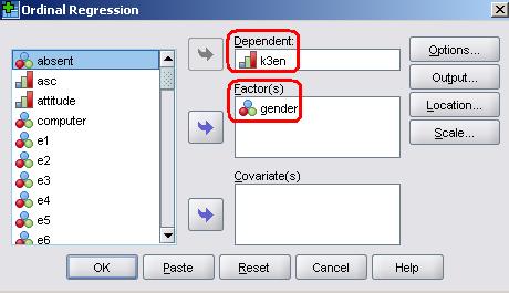
You access the menu via: Analyses > Regression > Ordinal. The window shown below opens. Move English level (k3en) to the ‘Dependent’ box and gender to the ‘Factor(s)’ box.

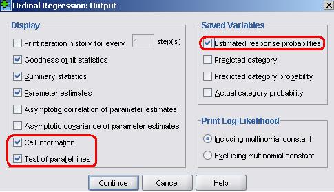
Next click on the Output button. Here we can specify additional outputs. Place a tick in Cell Information. For relatively simple models with a few factors this can help in evaluating the model. However, this is not recommended for models with many factors or for models with continuous covariates, since such models typically result in very large tables which are often of limited value in evaluating the model because they are so extensive (they are so extensive, in fact, that they are likely to cause severe mental distress). Also place a tick in the Test of parallel lines box. This is essential as it will ask SPSS to perform a test of the proportional odds (or parallel lines) assumption underlying the ordinal model (see Page 5.3).

You also see here options to save new variables (see under the ‘Saved Variables’ heading) back to your SPSS data file. This can be particularly useful during model diagnostics. Put a tick in the Estimated response probabilities box. This will save, for each case in the data file, the predicted probability of achieving each outcome category, in this case the estimated probabilities of the student achieving each of the levels (3, 4, 5, 6 and 7).

That is all we need to change in this example so click Continue to close the submenu and then OK on the main menu to run the analysis...

Examining the SPSS ordinal output

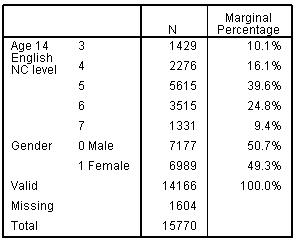
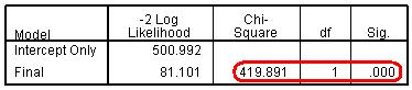
Several tables of thrilling numeric output will pour forth in to the output window. Let’s work through it together. Figure 5.4.1 shows the Case processing summary. SPSS clearly labels the variables and their values for the variables included in the analysis. This is important to check you are analysing the variables you want to. Here I can see we are modelling KS3 English level in relation to gender (with girls coded 1).

Figure 5.4.1: Case Processing Summary

Figure 5.4.2 shows the Model fitting information. Before we start looking at the effects of each explanatory variable in the model, we need to determine whether the model improves our ability to predict the outcome. We do this by comparing a model without any explanatory variables (the baseline or ‘Intercept Only’ model) against the model with all the explanatory variables (the ‘Final’ model - this would normally have several explanatory variables but at the moment it just contains gender). We compare the final model against the baseline to see whether it has significantly improved the fit to the data. The Model fitting Information table gives the -2 log-likelihood (-2LL, see Page 4.6) values for the baseline and the final model, and SPSS performs a chi-square to test the difference between the -2LL for the two models.

Figure 5.4.2: Model Fit

The statistically significant chi-square statistic (p<.0005) indicates that the Final model gives a significant improvement over the baseline intercept-only model. This tells you that the model gives better predictions than if you just guessed based on the marginal probabilities for the outcome categories.

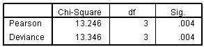
The next table in the output is the Goodness-of-Fit table (Figure 5.4.3). This table contains Pearson's chi-square statistic for the model (as well as another chi-square statistic based on the deviance). These statistics are intended to test whether the observed data are consistent with the fitted model. We start from the null hypothesis that the fit is good. If we do not reject this hypothesis (i.e. if the p value is large), then you conclude that the data and the model predictions are similar and that you have a good model. However if you reject the assumption of a good fit, conventionally if p<.05, then the model does not fit the data well. The results for our analysis suggest the model does not fit very well (p<.004). 

Figure 5.4.3: Goodness of fit test

We need to take care not to be too dogmatic in our application of the p<.05 rule. For example the chi-square is highly likely to be significant when your sample size is large, as it certainly is with our LSYPE sample of roughly 15,000 cases. In such circumstances we may want to set a lower p-value for rejecting the assumption of a good fit, maybe p<.01. More importantly, although the chi-square can be very useful for models with a small number of categorical explanatory variables, they are very sensitive to empty cells. When estimating models with a large number of categorical (nominal or ordinal) predictors or with continuous covariates, there are often many empty cells (as we shall see later). You shouldn't rely on these test statistics with such models. Other methods of indexing the goodness of fit, such as measures of association, like the pseudo R², are advised.

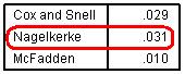
In linear regression, R² (the coefficient of determination) summarizes the proportion of variance in the outcome that can be accounted for by the explanatory variables, with larger R² values indicating that more of the variation in the outcome can be explained up to a maximum of 1 (see Module 2 and Module 3). For logistic and ordinal regression models it not possible to compute the same R² statistic as in linear regression so three approximations are computed instead (see Figure 5.4.4). You will remember these from Module 4 as they are the same as those calculated for logistic regression.

Figure 5.4.4: Pseudo R-square Statistics

What constitutes a “good” R² value depends upon the nature of the outcome and the explanatory variables. Here, the pseudo R² values (e.g. Nagelkerke = 3.1%) indicates that gender explains a relatively small proportion of the variation between students in their attainment. This is just as we would expect because there are numerous student, family and school characteristics that impact on student attainment, many of which will be much more important predictors of attainment than any simple association with gender. The low R² indicates that a model containing only gender is likely to be a poor predictor of the outcome for any particular individual student. Note though that this does not negate the fact that there is a statistically significant and relatively large difference in the average English level achieved by girls and boys.

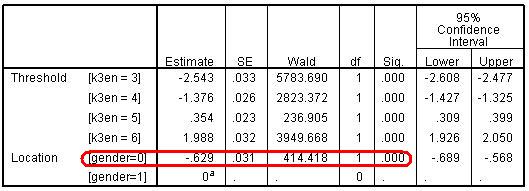
The Parameter estimates table (Figure 5.4.5) is the core of the output, telling us specifically about the relationship between our explanatory variables and the outcome.

Figure 5.4.5: Parameter Estimates Table

The threshold coefficients are not usually interpreted individually. They just represent the intercepts, specifically the point (in terms of a logit) where students might be predicted into the higher categories. The labelling may seem strange, but remember the odds of being level 6 or below (k3en=6) is just the complement of the odds of being level 7; the odds of being level 5 or below (k3en=5) are just the complement of the odds of being level 6 or above, and so on. While you do not usually have to interpret these threshold parameters directly we will explain below what is happening here so you understand how the model works. The results of our calculations are shown in Figure 5.4.6.

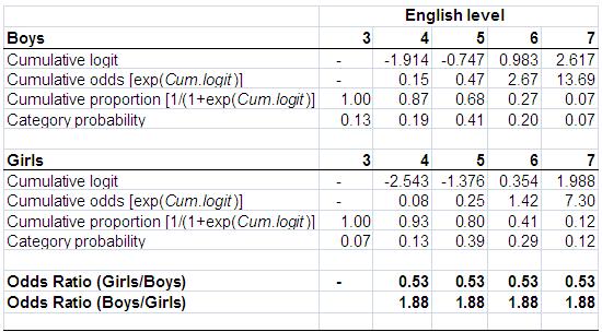
Let’s start with girls. Since girls represent our base or reference category the cumulative logits for girls are simply the threshold coefficients printed in the SPSS output (k3en = 3, 4, 5, 6). We take the exponential of the logits to give the cumulative odds (co) for girls. Note that these do not match the cumulative logits and odds we showed in Figure 5.3.3 because, as explained above, SPSS creates these as the odds for achieving each level or below as opposed to each level or above and because the reference category is boys not girls. However once these logits are converted to cumulative proportions/probabilities you can see they are broadly equivalent in the two tables (bar some small differences arising from the assumption of proportional odds in the ordinal model, more on which later). We calculate the predicted cumulative probabilities from the cumulative odds (co) simply by the formula 1/(1+co). If we want to find the predicted probability of being in a specific outcome category (e.g., at a specific English level) we can work out the category probability by subtraction. So if the probability of being at level 7 is 0.12 (or 12%), and the probability of being at level 6 or above is 0.41 (or 41%), then the probability of being specifically at level 6 is .41 - .12 = .29 (or 29%). Similarly the predicted probability for being specifically at Level 5 for girls is .80 - .41 = .39 (39%) and at level 4 it is .93 - .80 = .13 (13%). Finally the probability of being at level 3 is 1 - .93 = .07 (7%).

Figure 5.4.6: Parameters from the ordinal regression of gender on English level

To calculate the figures for boys (gender=0) we have to combine the parameters for the thresholds with the gender parameter (-.629, see Figure 5.4.5). Usually in regression we add the coefficient for our explanatory variable to the intercept to obtain the predicted outcome (e.g. y = a + bx, see modules 2 & 3). However in SPSS ordinal regression the model is parameterised as y = a - bx. This doesn’t make any difference to the predicted values, but is done so that positive coefficients tell you that higher values of the explanatory variable are associated with higher outcomes, while negative coefficients tell you that higher values of the explanatory variable are associated with lower outcomes. So for example the cumulative logit for boys at ‘level 4+’ is -2.543 - (-.629) = -1.914, at level 5+ it is -1.376 - (-.629) = -.747 and so on. Then, just as for girls, the cumulative odds (co) are the exponent of the logits, the cumulative proportions are calculated as 1/(1+co), and the category probabilities are found by subtraction in the same way as described for girls. Phew!

Odds Ratios

We can divide the odds for girls by the odds for boys at each cumulative split to give the OR (see Figure 5.4.6). We can see that in the proportional odds model the OR is constant (0.53) at all cumulative splits in the data (the odds of boys achieving a higher level are approximately half the odds for girls). We can express the OR the other way round by dividing the odds for boys by the odds for girls which gives us the OR of 1.88 (the odds for girls of achieving a higher level are approximately twice the odds for boys). As we saw in Module 4 these OR of 0.53 and 1.88 are equivalent, they just vary depending on the reference category. (see Extension D - you can convert an OR to its complement by dividing the OR into 1, e.g. 1/0.53= 1.88, equally 1/1.88=0.53). The important thing to note here is that the gender OR is consistent at each of the cumulative splits in the distribution.

The above was completed just to demonstrate the proportional odds principle underlying the ordinal model. In fact we do not have to directly calculate the ORs at each threshold as they are summarised in the parameter for gender. This shows the estimated coefficient for gender is -.629 and we take the exponent of this to find the OR with girls as the base: exp(-.629) = 0.53. To find the complementary OR with boys as the base just reverse the sign of the coefficient before taking the exponent, exp(.629)=1.88. The interpretation of these ORs is as stated above.

Test of parallel lines

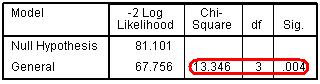
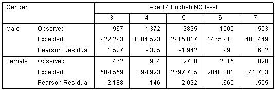
Remember that the OR is equal at each threshold because the ordinal model has constrained it to be so through the proportional odds (PO) assumption. We can evaluate the appropriateness of this assumption through the ‘test of parallel lines’. This test compares the ordinal model which has one set of coefficients for all thresholds (labelled Null Hypothesis), to a model with a separate set of coefficients for each threshold (labelled General). If the general model gives a significantly better fit to the data than the ordinal (proportional odds) model (i.e. if p<.05) then we are led to reject the assumption of proportional odds. This is the conclusion we would draw for our example (see Figure 5.5.7), given the significant value as shown below (p<.004).

Figure 5.4.7: Test of Parallel Lines

Note: The sharp-eyed among you may have noted that the chi-square statistics given above for the Test of Parallel Lines is exactly the same as that given for the omnibus test of the ‘goodness of fit’ of the whole model. This is because we have only a single explanatory variable in our model, so the two tests are the same. However when we have multiple explanatory variables this will not be the case.

We can see why this is the case if we compare our OR from the ordinal regression to the separate ORs calculated at each threshold in Figure 5.3.3. While the odds for boys are consistently lower than the odds for girls, the OR from the ordinal regression (0.53) underestimates the extent of the gender gap at the very lowest level (Level 4+ OR = 0.45) and slightly overestimates the actual gap at the highest level (level 7 OR =.56). We see how this results in the significant chi-square statistic in the ‘test for parallel lines’ if we compare the ‘observed’ and ‘expected’ values in the ‘cell information’ table you requested, shown below as Figure 5.4.8. The use of the single OR in the ordinal model leads to predicting fewer boys and more girls at level 3 than is actually the case (shown by comparing the ‘expected’ numbers from the model against the ‘observed’ numbers).

Figure 5.4.8: Output for Cell Information

However the test of the proportional odds assumption has been described as anti-conservative, that is it nearly always results in rejection of the proportional odds assumption (O’Connell, 2006, p.29) particularly when the number of explanatory variables is large (Brant, 1990), the sample size is large (Allison, 1999; Clogg & Shihadeh, 1994) or there is a continuous explanatory variable in the model (Allison, 1999). It is advisable to examine the data using a set of separate logistic regression equations to explicitly see how the ORs vary at the different thresholds, as we have done in Figure 5.3.3. In this particular case it might be reasonable to conclude that the OR for gender from the PO model (0.53) - while it does underestimate the extent of the over-representation of boys at the lowest level - does not differ hugely from those of the separate logistic regressions (0.45-0.56) and so is a reasonable summary of the trend across the data. Here the statistical test that led to the rejection of the PO assumption probably reflects the large sample size in our LSYPE dataset.

Predicted probabilities

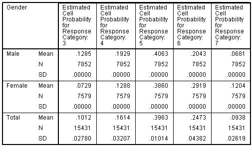
Figure 5.4.6 showed how from the model we can calculate the cumulative proportion at each threshold and, by subtraction, the predicted probability of being at any specific level. However you don’t actual have to do any of these calculations to determine the predicted probabilities since we requested SPSS to save the estimated probabilities for each case. We have five possible outcomes (level 3 to level 7) so SPSS will save the predicted probabilities for each case in five new variables that by default will be labelled EST1_1 to EST5_1. The first number refers to the category where 1 will indicate the lowest value for our ordinal outcome (i.e. level 3) and 5 will indicate the highest value (i.e. level 7). The second number after the underscore (_1) indicates these are the predictions from the first model we have run. If we added some more explanatory variables and ran a second model, without first deleting the variables holding estimated probabilities from the first model, then the predictions from the second model would have the suffix _2, i.e. EST1_2, EST2_2, EST3_2 etc. If you do intend to run multiple models it may be worth renaming these variables or labelling them carefully so that you do not lose track!

We can use these estimates to explore the predicted probabilities in relation to our explanatory variables. For example we can use the MEANS command (Analyze>Compare Means>Means) to report on the estimated probabilities of being at each level for boys and girls. The output is shown below (Figure 5.4.9):

Figure 5.4.9: Estimated probabilities for boys and girls from the ordinal regression

Note: the SD is zero in all cells because, with gender being the only explanatory variable in the model, all males will have the same predicted probabilities within each outcome category, and all females will also have the same predicted probabilities within each outcome category.

The ability to summarise and plot these predicted probabilities will be quite useful later on when we have several explanatory variables in our model and want to visualise their associations with the outcome.  

Summary

We have seen that where we have an ordinal outcome there is value in trying to summarise the outcome in a single model, rather than completing several separate logistic regression models. However we have also seen that this can overly simplify the data and it is important to complete the separate logistic models to fully understand the nuances in our data. For example, here the ordinal (PO) model did not identify the true extent to which boys were over-represented relative to girls at the lowest level. We should always complete separate logistic regressions if the assumption of PO is rejected. In the particular example used here it might be reasonable to conclude that the OR for gender from the ordinal (PO) model (0.53) does not differ hugely from those of the separate logistic regressions (0.45-0.56) and so is a reasonable summary of the trend across the data. However you are only in a position to conclude this if you have completed the separate logistic models, so in practice our advice is always to do the separate logistic models when the PO assumption is formally rejected. Given the anti-conservative nature of the test of the proportional odds assumption (O’Connell, 2006) this will more often than not be the case. Let us now move on to consider models which have more than one explanatory variable.

Navigation

Home
Modules
Site Guide
Module 5 Contents
Resources