Question 1 This question can be answered by creating a frequency table (head to the Foundation Module if you have forgotten how to do this).

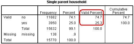As you can see just over 25% of the students in the sample come from a single parent home.

 

Question 2 This question requires a crosstabulation with chi-square analysis. If you are rusty on this head over to Page 2.2.

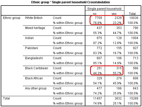The table shows that the percentage of those from a single parent family does indeed vary between ethnic groups. For example, about 23% of the students from White British backgrounds are from single parent households compared to nearly 56% of those from Black Caribbean backgrounds. We can test the statistical significance of this association using chi-square.

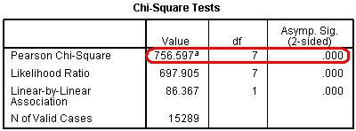As the test shows, the chi-square value of 756.6 is statistically significant (p < .005) so it is unlikely that an association of this strength could have occurred in our sample if there was no such association in the overall population.

 

Question 3 A bar chart which uses the mean of the age 14 exam scores (ks2stand) on the y-axis is best for answering this question. If you can’t quite recall how to do this the process is described in the Foundation Module.

 

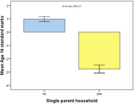As you can see, the mean age 14 score for students from single parent families is substantially lower than average while those from backgrounds with two parents score slightly higher than average. We have added error bars to our chart to ascertain how confident we can feel with regard to the accuracy of our calculated mean scores.

 

Question 4You will need to re-run model 7 (on Page 3.13) but add the single parent family (singlepar) variable as an explanatory variable. The basic procedures for running a regression module start on Page 3.4. The table required for answering this question is the coefficients table:

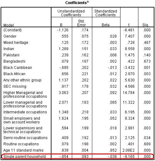We have highlighted the single parent family variable. The columns marked t and sig test tell us that the variable is contributing to the model to a statistically significant degree (p < .005). The B-coefficient in the first column suggests that, even after all the other variables in the model are held constant, those students from single parent families score an average of -.854 less standard marks at age 14 than their peers from families with two parents. Though this is significant, the Beta column puts this in perspective by providing a standardised coefficient for all variables. The Beta value of -.038 is much smaller than the one for age 11 exam score (.852) which shows that prior attainment is a more powerful predictor of exam score by far.

 

Question 5 Answering this question requires you to break the model down in to two blocks, with the first block being the original model 7 and the second block being model 7 plus the single parent family variable. You will also need to request R-square change statistics from SPSS. The process for doing both of these things is explained at the end of Page 3.11. The Model Summary is shown below, complete with R-Square Change statistics.

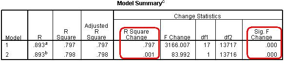The highlighted R square Change column for ‘model 2’ (where singlepar was added) shows that the r² only increases by .001 compared to the original model 7 (labelled ‘1’ here – just to confuse you!). This means that only an additional 0.1% of variance in age 14 exam score was explained by the new model. This is a small amount but that does not mean it is not a significant amount. The Sig. F Change indicates that the enhanced model (‘2’) is better at predicting the outcome to its predecessor (‘1’) to a statistically significant level (p < .005).

 

Question 6 To check this assumption you will need to examine a scatterplot which has the standardised predicted values for each participant on the x-axis and the standardised residual for each participant on the y-axis. This is achieved using the Plots submenu on the right hand side of the main regression window. Pages 3.3 and 3.14 discuss assumptions and how to test them if you are unsure how to do this.

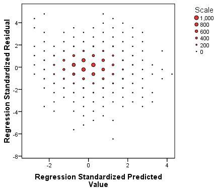The plot looks relatively unchanged from the one we saw when running diagnostics on model 7 (Page 3.14). The points are spread out in a fairly random manner which suggests that our assumption of homoscedasticity is likely to be safe!

Navigation

Home
Modules
Site Guide
Module 3 Contents
Resources