On Page 4.9 we discussed the assumptions and issues involved with logistic regression and were relieved to find that they were largely familiar to us from when we tackled multiple linear regression! Despite this, testing them can be rather tricky. We will now show you how to perform these diagnostics using SPSS based on the model we used as an example on Page 4.11 (using the MLR LSYPE 15,000 dataset ).

Linearity of Logit

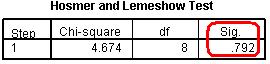
This assumption is confusing but it is not usually an issue. Problems with the linearity of the logit can usually be identified by looking at the model fit and pseudo R² statistics (Nagelkerke R², see Page 4.12 - Figure 4.12.4). The Hosmer and Lemeshow test, which as you may recall was discussed on Page 4.12 and shown as SPSS output in Figure 4.12.5 (reprinted below) is a good test of how well your model fits the data. If the test is not statistically significant (as is the case with our model here!) you can be fairly confident that you have fitted a good model.

Figure 4.14.1: Hosmer and Lemeshow Test

With regard to the Nagelkerke R² you are really just checking that your model is explaining a reasonable amount of the variance in the data. Though in this case the value of .159 (about 16%) is not high in absolute terms it is highly statistically significant.

Of course this approach is not perfect. Field (2009, p.296, see Resources) suggests an altogether more technical approach to testing the linearity of the logit if you wish to have more confidence that your model is not violating its assumptions.

Independent Errors

As we mentioned on Page 4.9 checking for this assumption is only really necessary when data is clustered hierarchically and this is beyond the scope of this website. We thoroughly recommend our sister site LEMMA (see Resources) if you want to learn more about this.

Multicollinearity

It is important to know how to perform the diagnostics if you believe there might be a problem. The first thing to do is simply create a correlation matrix and look for high coefficients (those above .8 may be worthy of closer scrutiny). You can do this very simply on SPSS: Analyse > Correlate > Bivariate will open up a menu with a single window and all you have to do is add all of the relevant explanatory variables into it and click OK to produce a correlation matrix.

If you are after more detailed colinearity diagnostics it is unfortunate that SPSS does not make it easy to perform them when creating a logistic regression model (such a shame, it was doing so well after including the ‘interaction’ button). However, if you recall, it is possible to collect such diagnostics using the menus for multiple linear regression (see Page 3.14)… because the tests of multicollinearity are actually independent of the type of regression model you are making (they examine only the explanatory variables) you can get them from running a multiple linear regression using the exact same variables as you used for your logistic regression. Most of the output will be meaningless because the outcome variable is not continuous (which violates a key assumption of linear regression methods) but the multicollinearity diagnostics will be fine! Of course we have discussed this whole issue in the previous module (Page 3.14).

Influential Cases

On page 4.11 we showed you how to request the model’s residuals and the Cook’s distances as new variables for analysis. As you may recall from the previous module (Page 3.14), if a case has a Cook’s distance greater than one it may be unduly influencing your model. Requesting the Cook’s distance will have created a new variable in your dataset called COO_1 (note that this might be different if you have created other variables in previous exercises – this is why clearly labelling variables is so useful!). To check that we have no cases where Cook’s distance is greater than one we can simply look at the frequencies: Analyse > Descriptive Statistics > Frequencies, add Coo_1 into the window, and click OK. Your output, terrifyingly, will look something like Figure 4.14.2 (only much, much longer!):

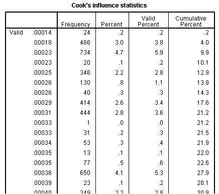
Figure 4.14.2: Frequency of Cook’s distance for model

This is not so bad though – remember we are looking for values greater than one and these values are in order. If you scroll all the way to the bottom of the table you will see that the highest value Cook’s distance is less than .014… nowhere near the level of 1 at which we need to be concerned.

Finally we have reached the end of our journey through the world of Logistic Regression. Let us now take stock and discuss how you might go about pulling all of this together and reporting it.

Navigation

Home
Modules
Site Guide
Module 4 Contents
Resources