Key Assumptions
You will find that the assumptions for logistic regression are very similar to the assumptions for linear regression. If you need a recap, rather than boring you by repeating ourselves like statistically obsessed parrots (the worst kind of parrot) we direct you to our multiple regression assumptions on Page 3.3 . However, there are still three key assumptions which you should be aware of:
- Linearity (sort of...): For linear regression the assumption is that the outcome variable has a linear relationship with the explanatory variables, but for logistic regression this is not possible because the outcome is binary. The assumption of linearity in logistic regression is that any explanatory variables have a linear relationship with the logit of the outcome variable. ‘What are they on about now?’ we imagine you’re sighing. If the relationship between the log odds of the outcome occurring and each of the explanatory variables is not linear than our model will not be accurate. We’ll discuss how to evaluate this in the context of SPSS over the coming pages, but the best way to check that the model you are creating is sensible is by looking at the model fit statistics and pseudo R2. If you are struggling with the concept of logits and log odds you can revise Pages 4.2 and 4.4 of this module.
- Independent errors: Identical to linear regression, the assumption of independent errors states that errors should not be correlated for two observations. As we said before in the simple linear regression module, this assumption can often be violated in educational research where pupils are clustered together in a hierarchical structure. For example, pupils are clustered within classes and classes are clustered within schools. This means students within the same school often have a tendency to be more similar to each other than students drawn from different schools. Pupils learn in schools and characteristics of their schools, such as the school ethos, the quality of teachers and the ability of other pupils in the school, may affect their attainment. In large scale studies like the LSYPE such clustering can to some extent be taken care of by using design weights which indicate the probability with which an individual case was likely to be selected within the sample. Thus published analyses of LSYPE (see Resources Page) specify school as a cluster variable and apply published design weights using the SPSS complex samples module. More generally researchers can control for clustering through the use of multilevel regression models (also called hierarchical linear models, mixed models, random effects or variance component models) which explicitly recognise the hierarchical structure that may be present in your data. Sounds complicated, right? It definitely can be and these issues are more complicated than we need here where we are focusing on understanding the essentials of logistic regression. However if you feel you want to develop these skills we have an excellent sister website provided by another NCRM supported node called LEMMA which explicitly provides training on using multilevel modelling including for logistic regression. We also know of some good introductory texts on multilevel modelling and you can find all of this among our Resources.
- Multicollinearity: This is also identical to multiple regression. The assumption requires that explanatory variables should not be highly correlated with each other. Of course they are often correlated with each other to some degree. As an example, below is a correlation matrix (Figure 4.9.1) that shows the relationships between several LSYPE variables.
Figure 4.9.1: Correlation Matrix – searching for multicollinearity issues
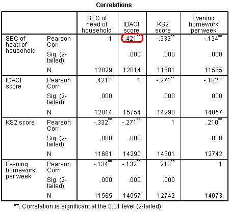
As you might expect, IDACI (Income Deprivation Affecting Children Index) is significantly related to the SEC (socio-economic classification) of the head of the household but the relationship does not appear strong enough (Pearson’s r = .42) to be considered a problem. Usually values of r = .8 or more are cause for concern. As before the Variance Inflation Factor (VIF) and tolerance statistics can be used to help you verify that multicollinearity is not a problem (see Page 3.3).


