The Deviance (-2LL) statistic

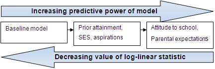
We will need to ascertain how good our regression model is once we have fitted it to the data – does it accurately explain the data, or does it incorrectly classify cases as often as it correctly classifies them? The deviance, or -2 log-likelihood (-2LL) statistic, can help us here. The deviance is basically a measure of how much unexplained variation there is in our logistic regression model – the higher the value the less accurate the model. It compares the difference in probability between the predicted outcome and the actual outcome for each case and sums these differences together to provide a measure of the total error in the model. This is similar in purpose to looking at the total of the residuals (the sum of squares) in linear regression analysis in that it provides us with an indication of how good our model is at predicting the outcome. The -2LL statistic (often called the deviance) is an indicator of how much unexplained information there is after the model has been fitted, with large values of -2LL indicating poorly fitting models. Don’t worry about the technicalities of this – as long as you understand the basic premise you’ll be okay!

The deviance has little intuitive meaning because it depends on the sample size and the number of parameters in the model as well as on the goodness of fit. We therefore need a standard to help us evaluate its relative size. One way to interpret the size of the deviance is to compare the value for our model against a ‘baseline’ model. In linear regression we have seen how SPSS performs an ANOVA to test whether or not the model is better at predicting the outcome than simply using the mean of the outcome. The change in the -2LL statistic can be used to do something similar: to test whether the model is significantly more accurate than simply always guessing that the outcome will be the more common of the two categories. We use this as the baseline because in the absence of any explanatory variables the ‘best guess’ will be the category with the largest number of cases.

Let’s clarify this with our fiveem example. In our sample 46.3% of student achieve fiveem while 53.7% do not. The probability of picking at random a student who does not achieve the fiveem threshold is therefore slightly higher than the probability of picking a student who does. If you had to pick one student at random and guess whether they would achieve fiveem or not, what would you guess? Assuming you have no other information about them, it would be most logical to guess that they would not achieve fiveem – simply because a slight majority do not. This is the baseline model which we can test our later models against. This is also the logistic model when only the constant is included. If we then add explanatory variables to the model we can compute the improvement as follows:

X²= [-2LL (baseline)] - [-2LL (new)]

with degrees of freedom= k_baseline- k_new, where k is the number of parameters in each model.

If our new model explains the data better than the baseline model there should be a significant reduction in the deviance (-2LL) which can be tested against the chi-square distribution to give a p value. Don’t worry - SPSS will do this for you! However if you would like to learn more about the process you can go to Extension F.

The deviance statistic is useful for more than just comparing the model to the baseline - you can also compare different variations of your model to see if adding or removing certain explanatory variables will improve its predictive power (Figure 4.6.1)! If the deviance (-2LL) is decreasing to a statistically significant degree with each set of explanatory variables added to the model then it is improving at accurately predicting the outcome for each case.

Figure 4.6.1 Predictors of whether or not student goes to university R² equivalents for logistic regression

R² equivalents for logistic regression

Another way of evaluating the effectiveness of a regression model is to calculate how strong the relationship between the explanatory variable(s) and the outcome variable is. This was represented by the R² statistic in linear regression analysis. R², or rather a form of it, can also be calculated for logistic regression. However, somewhat confusingly there is more than one version! This is because the different versions are pseudo-R² statistics that approximate the amount of variance explained rather than calculate it precisely. Remember we are dealing with probabilities here! Despite this it can still sometimes be useful to examine them as a way of ascertaining the substantive value of your model.

The two versions most commonly used are Hosmer & Lemeshow’s R² and Nagelkerke’s R². Both describe the proportion of variance in the outcome that the model successfully explains. Like R² in multiple regression these values range between ‘0’ and ‘1’ with a value of ‘1’ suggesting that the model accounts for 100% of variance in the outcome and ‘0’ that it accounts for none of the variance. Be warned: they are calculated differently and may provide conflicting estimates! These statistics are readily available through SPSS and we’ll show you how to interpret them when we run through our examples over the next few pages.

Navigation

Home
Modules
Site Guide
Module 4 Contents
Resources