Why Create a Logistic Regression Model?

So we can see the associations between ethnic group, social class (SEC), gender and achievement quite clearly without the need for any fancy statistical analysis. Why would we want to get involved in logistic regression modelling? There are three rather good reasons:

• To evaluate the statistical significance of the above associations. Remember that this data represents only a sample (although a very large sample) from the population of all students in England (approximately 600,000 students in any one year group). Are the effects in the sample sufficiently large relative to their standard errors that they are likely to be true in the population?
• To gauge the effect of one explanatory variable (e.g. ethnicity) on the outcome variable when controlling for other variables also associated with the outcome (e.g. SEC and gender). Specifically we are interested here in what the OR for ethnicity looks like after we have controlled for differences in exam achievement associated with SEC and gender.
• To gauge the extent and significance of any interactions between the explanatory variables in their effects on the outcome.

To do this we will need to run a logistic regression which will attempt to predict the outcome fiveem based on a student’s ethnic group, SEC and gender.

Setting up the logistic regression model

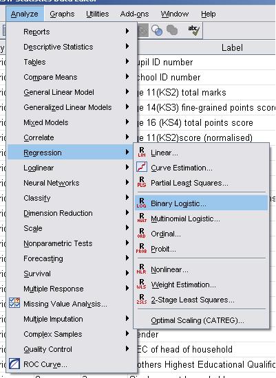
Let’s get started by setting up the logistic regression analysis. We will create a logistic regression model with three explanatory variables (ethnic, SEC and gender) and one outcome (fiveem) – this should help us get used to things! You can open up the LSYPE 15,000 Dataset to work through this example with us. You can also follow the process using our video demonstration .

Take the following route through SPSS: Analyse> Regression > Binary Logistic

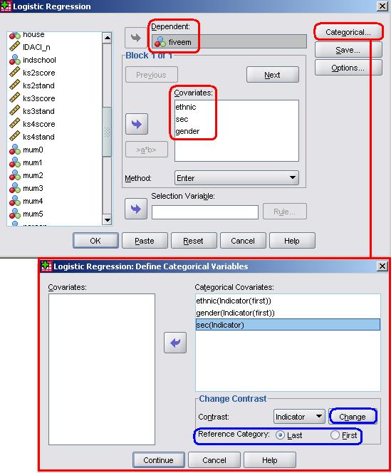
The logistic regression pop-up box will appear and allow you to input the variables as you see fit and also to activate certain optional features. First of all we should tell SPSS which variables we want to examine. Our outcome measure is whether or not the student achieves five or more A*-Cs (including Maths and English) and is coded as ‘0’ for no and ‘1’ for yes. This variable is labelled fiveem and should be moved in to the Dependent box.

Any explanatory variables need to be placed in what is named the covariates box. If the explanatory variable is continuous it can be dropped in to this box as normal and SPSS can be trusted to add it to the model, However, the process is slightly more demanding for categorical variables such as the three we wish to add because we need to tell SPSS to set up dummy variables based on a specific baseline category (we do not need to create the dummies ourselves this time… hooray!).

Let’s run through this process. To start with, move ethnic, SEC and Gender into the covariates box. Now they are there we now need to define them as categorical variables. To do this we need to click the button marked ‘Categorical’ (a rare moment of simplicity from our dear friend SPSS) to open a submenu. You need to move all of the explanatory variables that are categorical from the left hand list (Covariates) to the right hand window… in this case we need to move all of them!

The next step is to tell SPSS which category is the reference (or baseline) category for each variable. To do this we must click on each in turn and use the controls on the bottom right of the menu which are marked ‘Change Contrast’. The first thing to note is the little drop down menu which is set to ‘Indicator’ as a default. This allows you to alter how categories within variables are compared in a number of ways (that you may or may not be pleased to hear are beyond the scope of this module). For our purposes we can stick with the default of ‘indicator’, which essentially creates dummy variables for each category to compare against a specified reference category – a process which you are probably getting familiar with now (if not, head to Page 3.6).

All we need to do then is tell SPSS whether the first or last category should be used as the reference and then click ‘Change’ to finalise the setting. For our Ethnic variable the first category is ‘0’ White-British (the category with the highest number of participants) so, as before, we will use this as the reference category. Change the selection to ‘First’ and click ‘Change’. For the Gender variable we only have two categories and could use either male (‘0’) or female (‘1’) as the reference. Previously we have used male as the reference so we will stick with this (once again, change the selection to ‘First’ and click ‘Change’). Finally, for Socio Economic Class (sec) we will use the least affluent class as the reference (‘Never worked/long term unemployed - 8’). This time we will use the ‘Last’ option given that the SEC categories are coded such that the least affluent one is assigned the highest value code. Remember to click ‘Change’! You will see that your selections have appeared in brackets next to each variable and you can click ‘Continue’ to close the submenu.

Notice that on the main Logistic Regression menu you can change the option for which method you use with a drop down menu below the covariates box. As we are entering all three explanatory variables together as one block you can leave this as ‘Enter’. You will also notice that our explanatory variables (Covariates) now have ‘Cat’ printed next to them in brackets. This simply means that they have been defined as categorical variables, not that they have suddenly become feline (that would just be silly).

The Logistic Regression Sub-menus

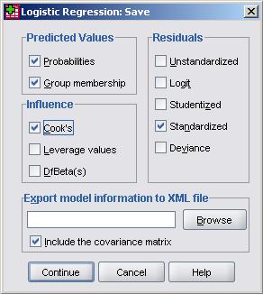
Now that our variables have been defined we can start playing with the option menus. Beware SPSS’s desire to dazzle you with a myriad of different tick boxes, options and settings - some people just like to show off! We’ll guide you through the useful options. The save sub-menu is very useful and can be seen below.

If you recall, the save options actually create new variables for your data set. We can ask SPSS to calculate four additional variables for us:

Predicted probabilities – This creates a new variable that tells us for each case the predicted probability that the outcome will occur (that fiveem will be achieved) based on the model.

Predicted Group Membership – This new variable estimates the outcome for each participant based on their predicted probability. If the predicted probability is >0.5 then they are predicted to achieve the outcome, if it is <.5 they are predicted not to achieve the outcome. This .5 cut-point can be changed, but it is sensible to leave it at the default. The predicted classification is useful for comparison with the actual outcome!

Residuals (standardised) – This provides the residual for each participant (in terms of standard deviations for ease of interpretation). This shows us the difference between the actual outcome (0 or 1) and the probability of the predicted outcome and is therefore a useful measure of error.

Cook’s – We’ve come across this in our travels before. This generates a statistic called Cook’s distance for each participant which is useful for spotting cases which unduly influence the model (a value greater than ‘1’ usually warrants further investigation).

The other options can be useful for the statistically-minded but for the purposes of our analysis the options above should suffice (we think we are fairly thorough!). Click on Continue to shut the sub-menu. The next sub-menu to consider is called options:

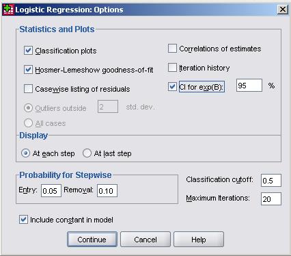
Again we have highlighted a few of the options here:

Classification plots – Checking this option requests a chart which shows the distribution of outcomes over the probability range (classification plot). This is useful for visually identifying where the model makes most incorrect categorizations. This will make more sense when we look at one on the Page 4.12!

Hosmer-Lemeshow Goodness of fit – This option provides a X² (Chi-square) test of whether or not the model is an adequate fit to the data. The null hypothesis is that the model is a ‘good enough’ fit to the data and we will only reject this null hypothesis (i.e. decide it is a ‘poor’ fit) if there are sufficiently strong grounds to do so (conventionally if p<.05). We will see that with very large samples as we have here there can be problems with this level of significance, but more on that later.

CI for exp(B) – CI stands for confidence interval and this option requests the range of values that we are confident that each odds ratio lies within. The setting of 95% means that there is only a p < .05 that the value for the odds ratio, exp(B), lies outside the calculated range (you can change the 95% confidence level if you are a control freak!).

Click on continue to close the sub-menu. Once you are happy with all the settings take a deep breath... and click OK to run the analysis.

Navigation

Home
Modules
Site Guide
Module 4 Contents
Resources