-
- Mod 4 - Log Reg
- 4.1 Overview
- 4.2 Odds, Odds Ratios and Exponents
- Quiz A
- 4.3 A General Model
- 4.4 Log Reg Model
- 4.5 Logistic Equations
- 4.6 How good is the model?
- 4.7 Multiple Explanatory Variables
- 4.8 Methods of Log Reg
- 4.9 Assumptions
- 4.10 Example from LSYPE
- 4.11 Log Reg on SPSS
- 4.12 SPSS Log Reg Output
- 4.13 Interaction Effects
- 4.14 Model Diagnostics
- 4.15 Reporting the Results
- Quiz B
- Exercise
- Mod 4 - Log Reg
Using Statistical Regression Methods in Education Research

4.2 An Introduction to Odds, Odds Ratios and Exponents
|
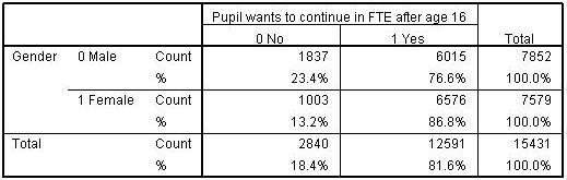
Let’s start by considering a simple association between two dichotomous variables (a 2 x 2 crosstabulation) drawing on the LSYPE dataset. The outcome we are interested in is whether students aspire to continue in Full-time education (FTE) after the age of 16 (the current age at which students in England can choose to leave FTE). We are interested in whether this outcome varies between boys and girls. We can present this as a simple crosstabulation (Figure 4.2.1). Figure 4.2.1: Aspiration to continue in full time education (FTE) after the age of 16 by gender: Cell counts and percentages We have coded not aspiring to continue in FTE after age 16 as 0 and aspiring to do so as 1. Although it is possible to code the variable with any values, employing the values 0 and 1 has advantages. The mean of the variable will equal the proportion of cases with the value 1 and can therefore be interpreted as a probability. Thus we can see that the percentage of all students who aspire to continue in FTE after age 16 is 81.6%. This is equivalent to saying that the probability of aspiring to continue in FTE in our sample is 0.816.
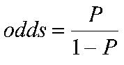
However another way of thinking of this is in terms of the odds. Odds express the likelihood of an event occurring relative to the likelihood of an event not occurring. In our sample of 15,431 students, 12,591 aspire to continue in FTE while 2,840 do not aspire, so the odds of aspiring are 12591/2840 = 4.43:1 (this means the ratio is 4.43 to 1, but we conventionally do not explicitly include the :1 as this is implied by the odds). The odds tell us that if we choose a student at random from the sample they are 4.43 times more likely to aspire to continue in FTE than not to aspire to continue in FTE. We don’t actually have to calculate the odds directly from the numbers of students if we know the proportion for whom the event occurs, since the odds of the event occurring can be gained directly from this proportion by the formula (Where p is the probability of the event occurring.):
Thus the odds in our example are: Odds= [p/(1-p)] = .816 / (1-.816 )= .816 /.184 = 4.43. The above are the unconditional odds, i.e. the odds in the sample as a whole. However odds become really useful when we are interested in how some other variable might affect our outcome. We consider here what the odds of aspiring to remain in FTE are separately for boys and girls, i.e. conditional on gender. We have seen the odds of the event can be gained directly from the proportion by the formula odds=p/(1-p). So for boys the odds of aspiring to continue in FTE = .766/(1-.766)= 3.27 While for girls the odds of aspiring to continue in FTE = .868/(1-.868)= 6.56. These are the conditional odds, i.e. the odds depending on the condition of gender, either boy or girl. We can see the odds of girls aspiring to continue in FTE are higher than for boys. We can in fact directly compare the odds for boys and the odds for girls by dividing one by the other to give the Odds Ratio (OR). If the odds were the same for boys and for girls then we would have an odds ratio of 1. If however the odds differ then the OR will depart from 1. In our example the odds for girls are 6.53 and the odds for boys are 3.27 so the OR= 6.56 / 3.27 = 2.002, or roughly 2:1. This says that girls are twice as likely as boys to aspire to continue in FTE. Note that the way odd-ratios are expressed depends on the baseline or comparison category. For gender we have coded boys=0 and girls =1, so the boys are our natural base group. However if we had taken girls as the base category, then the odds ratio would be 3.27 / 6.56= 0.50:1. This implies that boys are half as likely to aspire to continue in FTE as girls. You will note that saying “Girls are twice as likely to aspire as boys” is actually identical to saying “boys are half as likely to aspire as girls”. Both figures say the same thing but just differ in terms of the base. Odds Ratios from 0 to just below 1 indicate the event is less likely to happen in the comparison than in the base group, odds ratios of 1 indicate the event is exactly as likely to occur in the two groups, while odds ratios from just above 1 to infinity indicate the event is more likely to happen in the comparator than in the base group. Extension D
An interesting fact can be observed if we look at the odds for boys and the odds for girls in relation to the odds ratio (OR). For boys (our base group) the odds= 3.27 * 1 = 3.27 For girls the odds = 3.27 * 2.002 = 6.56. So another way of looking at this is that the odds for each gender can be expressed as a constant multiplied by a gender specific multiplicative factor (namely the OR). p/(1-p) = constant * OR. However there are problems in using ORs directly in any modelling because they are asymmetric. As we saw in our example above, an OR of 2.0 indicates the same relative ratio as an OR of 0.50, an OR of 3.0 indicates the same relative ratio as an OR of 0.33, an OR of 4.0 indicates the same relative ratio as an OR of 0.25 and so on. This asymmetry is unappealing because ideally the odds for males would be the opposite of the odds for females.
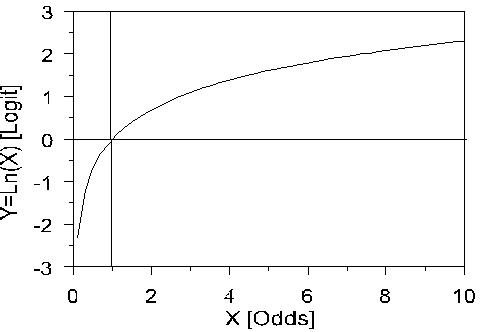
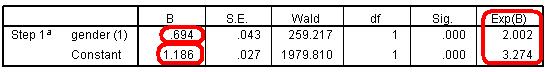
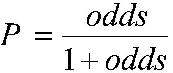
This asymmetry problem disappears if we take the ‘log’ of the odds ratio (OR). ‘Log’ doesn’t refer to some sort of statistical deforestation… rather a mathematical transformation of the odds which will help in creating a regression model. Taking the log of an OR of 2 gives the value Log(2)= +0.302 and taking the log of an OR of 0.50 gives the value Log (0.5)= -0.302. See what’s happened? The Log of the OR, sometimes called the logit (pronounced ‘LOH-jit’, word fans!) makes the relationships symmetric around zero (the OR’s become plus and minus .302). Logits and ORs contain the same information, but this difference in mathematical properties makes logits better building blocks for logistic regression. But what is a log function? How does it transform the ORs? Well, the natural log function looks like this (Figure 4.2.2): Figure 4.2.2: The natural log function So if we take the log of each side of the equation we can then express the log odds as: Log [p/(1-p)] = constant + log (OR) If the constant is labelled a, the log of the OR is labelled b, and the variable gender (x) takes the value 0 for boys and 1 for girls, then: Log [p/(1-p)] = a + bx Note that taking the log of the odds has converted this from a multiplicative to an additive relationship with the same form as the linear regression equations we have discussed in the previous two modules (it is not essential, but if you want to understand how logarithms do this it is explained in Extension E Log [p/(1-p)] = a + b1x1+ b2x2 + b3x3 + ... + bnxn. Output from a logistic regression of gender on educational aspiration If we use SPSS to complete a logistic regression (more on this later) using the student level data from which the summary Figure 4.2.1 was constructed, we get the logistic regression output shown below (Figure 4.2.3). Figure 4.2.3: Output from a logistic regression of gender on aspiration to continue in FTE post 16 Let’s explain what this output means. The B weights give the linear combination of the explanatory variables that best predict the log odds. So we can determine that the log odds for: Male: Log [p/(1-p)] = 1.186 + (0.694 * 0) = 1.186 Female: Log [p/(1-p)] = 1.186 + (0.694 * 1) = 1.880 The inverse of the log function is the exponential function, sometimes conveniently also called the anti-logarithm (nice and logical!). So if we want to convert the log odds back to odds we take the exponent of the log odds. So the odds for our example are: Male: Exp (1.186) = 3.27 Female: Exp (1.880) = 6.55 The odds ratio is given in the SPSS output for the gender variable [indicated as Exp(B)] showing that girls are twice as likely as boys to aspire to continue in FTE. By simple algebra we can rearrange the formula odds= [p/(1-p] to solve for probabilities:
Males: p= 3.27 / (1+3.27) = .766 Females: p= 6.55 / (1+6.55) = .868. These probabilities, odds and odds ratios - derived from the logistic regression model - are identical to those calculated directly from Figure 4.2.1. This is because we have just one explanatory variable (gender) and it has only two levels (girls and boys). This is called a saturated model for which the expected counts and the observed counts are identical. The logistic regression model will come into its own when we have an explanatory variable with more than two values, or where we have multiple explanatory variables. However what we hope this section has done is show you how probabilities, odds, and odds ratios are all related, how we can model the proportions in a binary outcome through a linear prediction of the log odds (or logits), and how these can be converted back into odds ratios for easier interpretation. Take the quiz to check you are comfortable with what you have learnt so far. If you are not perturbed by maths and formulae why not check out Extension E
|