Dichotomous explanatory variables

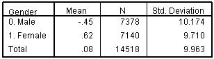
As discussed on the previous page, SEC can reasonably be treated as a scale, but what do we do with variables which are nominal? What if the categories cannot be placed in a rank order? Let us take the example of gender. Gender is usually a dichotomous variable – participants are either male or female. Figure 3.6.1 displays the mean age 14 standard scores for males and females in the sample. There is a difference of a whole score point between the scores of males and females, which suggests a case for adding gender to our regression model.

Figure 3.6.1: Mean age 14 score by gender

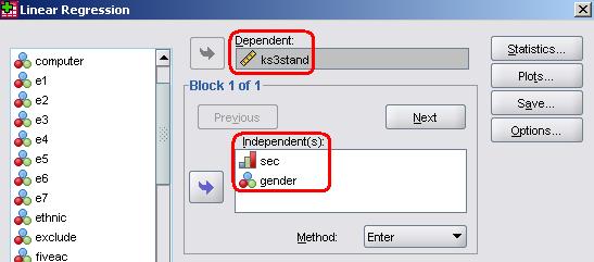
Take the following route through SPSS: Analyse> Regression > Linear. Add gender to the independents box – we are now repeating the multiple regression we performed on the previous page but adding gender as an explanatory variable. Do not worry about all of the extra options and assumptions yet – we will come to that later! Just click OK.

You will be starting to get familiar with these three tables now. 

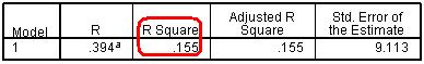
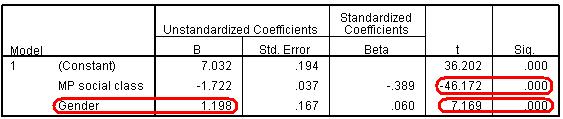
Figure 3.6.2: Multiple r and r² for model

Our Model Summary (Figure 3.6.2) tells us that our new model now has r² = .155 which suggests that 15.5% of the total variance in age 14 score can be explained. This is only very slightly more than the previous model (15.1%). But has the inclusion of gender made a significant contribution to explaining age 14 test score? We evaluate this through inspecting the coefficients table.

Figure 3.6.3: Coefficients for model

The Coefficient table (Figure 3.6.3) provides us with a fresh challenge: how do we interpret the b-coefficient for gender? Actually it is delightfully simple! If you recall the code ‘0’ was used for males and ‘1’ for females. The b-coefficient tells us how much higher or lower the category coded 1 (females) score in direct comparison to the category coded 0 (males) when the other variables in the model (currently SEC) are controlled (held fixed). The B coefficient for gender indicates that females score on average 1.2 standard marks higher than males, whatever the SEC of the home. The t-tests indicate that both explanatory variables are making a statistically significant contribution to the predictive power of the model.

What are the relative strengths of SEC and gender in predicting age 14 score? We cannot tell this directly from the coefficients since these are not expressed on a common scale. A one unit increase in SEC does not mean the same thing as a one unit increase in gender. We can get a rough estimate of their relative size by evaluating the difference across the full range for each explanatory variable, so the range for SEC is 7*-1.72 or 12.0 points, whereas the range for gender is just 1.2 points (girls versus boys). Another way of judging the relative importance of explanatory variables is through the Beta (β) weights in the fourth column. These are a standardised form of b which range between 0 and 1 and give a common metric which can be compared across all explanatory variables. The effects of SEC is large relative to gender, as can be seen by the relative difference in beta values (-.389 versus .060). Note you ignore the sign since this only indicates the direction, whether the explanatory variable is associated with an increase or decrease in outcome scores, it is the absolute value of Beta which is used to gauge its importance. You will remember this from comparing the strength of correlation coefficients which we completed in the Simple Linear Regression module (see Page 2.4). The results indicate that SEC is a more powerful predictor of age 14 score than gender, but both make a contribution to the explanation of variance in age 14 score.

Navigation

Home
Modules
Site Guide
Module 3 Contents
Resources