Minimising the effect of missing data

So far we have treated SEC as a continuous variable or scale. What are the implications of having done this? Treating a variable as a scale means that any case with a missing value on the variable is lost from the analysis. The frequency table for SEC was shown in Figure 3.4.2. A total of 2941 cases (18.6%) were missing a value for SEC, which is a high level of data loss.

One way of coping with this is to recode SEC into dummy variables, as we did with ethnic group (Page 3.7), and to explicitly include the ‘missing’ values as an extra category. This has several advantages, it:

• Prevents the loss of data that would come from omitting all cases with missing values, as happens when SEC is treated as a scale variable (excluding missing data in this way is known as ‘Listwise’ deletion)
• Allows for the direct modelling of missing data rather than imputing missing values, for example by mean substitution, which has its own interpretative problems
• Allows for non-linearity in the relationship between the ordinal categories and student attainment
• Can simplify the interpretation of the relationship between the predictor and the outcome, since we can directly contrast against a reference category (e.g. compare all SEC categories against long term unemployed)
• Can ensure a consistent base in terms of the sample size across a range of hierarchical regression models by retaining all cases (including those with missing values) as new explanatory variables are added.

We used the following syntax to change SEC into a series of dummy variables: Creating dummy variables for SEC . Note that the variable we have not created a dummy for (long-term unemployed) will be our reference category in the analysis. You don’t need to do this though as we have already prepared the dummy variables for you in the MLR LSYPE 15000 file . Aren’t we nice?

Interpreting the Model 4 output

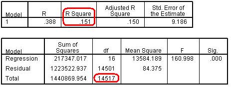
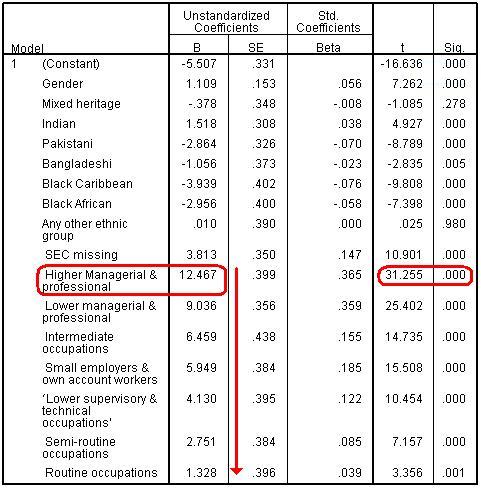
Repeat the regression we did on Page 3.7 using ks3stand as the Dependent variable and gender, e1 – e7 and sc0 – sc7 as the independent variables. Rather than assessing the effect of SEC as a regression coefficient we get a direct measure of how each category (including our ‘missing cases’ category) contrasts with the base category (long term unemployed).

Figure 3.9.1 presents the model summary and the ANOVA table. From the Model Summary we see that the model r² is 15.1%. This is lower than for model 3 where the model accounted for 17.0% of the variance. However this reflects two factors: the change from treating SEC as a scale variable to modelling it as a set of dummy variables and the increase in sample size associated with including the previously omitted 2,900 or so cases. We can see from the ANOVA table that we are including 14,518 cases in this analysis (the total df shows the number of cases - 1), rather than the 12,100 cases included in model 3. We will not pursue the relative contribution of these two factors here, since the increase in sample size is reason enough for preferring the treatment of SEC as a set of dummy variables.

Figure 3.9.1: model summary and the ANOVA table

Figure 3.9.2 shows the regression coefficients from the model.

Figure 3.9.2: Regression coefficients for Model 4

As we saw before, there is clearly a strong relationship between SEC and age 14 attainment, even after accounting for gender and ethnicity. Breaking the SEC variable down into its individual categories and comparing them to the base category of ‘long term unemployed’ makes interpretation of the coefficients more intuitive. For example, students from ‘Higher managerial and professional’ homes are predicted to obtain 12.5 more standard score marks than those from homes where the main parent is long term unemployed. Students from ‘lower managerial and professional’ homes achieve 9.0 more marks, those from intermediate homes 6.5 more marks and so on. You can see the ordinality in the data from the decreasing B coefficients: as the SEC of the home decreases there is a reduction in the extent of the ‘boost’ to age 14 standard score above the reference group of students from homes where the head of the household is long term unemployed. Being able to interpret the difference between categories in this way is very useful! We can see from the t statistic and associated ‘sig’ values that all SEC contrasts are highly statistically significant, including for those students with missing values for SEC.

Navigation

Home
Modules
Site Guide
Module 3 Contents
Resources