Interaction effects

So far we have considered only the main effects of each of our explanatory variables (SEC, gender and ethnic group) on attainment at age 14. That is we have evaluated the association of each factor with educational attainment while holding all other factors constant. This involves a strong assumption that the effects of SEC, gender and ethnic group are additive, that is there are no interactions between the effect of these variables. For example we have assumed that the ‘effect’ of SEC is the same for all ethnic groups, or equivalently that the ‘effect’ of ethnicity is the same at all levels of SEC. However there is the possibility that SEC and ethnic group may interact in terms of their effect on attainment, that the relationship between ethnicity and attainment may be different at different levels of SEC (or put the other way around that the relationship between SEC and attainment may vary for different ethnic groups, it’s the same thing). Is this assumption of additive effects valid, and how can we test it?

In any multiple linear regression model there exists the possibility of interaction effects. With only two explanatory variables there can of course be only one interaction, between explanatory variable 1 and explanatory variable 2, but the greater the number of variables in your model the higher the number of possible interactions. For example if we have 10 explanatory variables then there are 45 possible pairs of explanatory variables that may interact. It is unwieldy to test all possible combinations and indeed such ‘blanket testing’ may give rise to spurious effects, simply because at the 5% significance level some of the interactions might be statistically significant by chance alone. Your search for possible interactions should be guided by knowledge of the existing literature and theory in your field of study. In relation to the literature of educational attainment, there is quite strong emerging literature suggesting interactions between ethnicity and SEC (e.g. Strand, 1999; 2008). Let’s evaluate whether there is a statistically significant interaction between ethnicity and SEC in the current data, returning to the variables we used for model 3 (Page 3.7).

Step 1: Creating the interaction terms

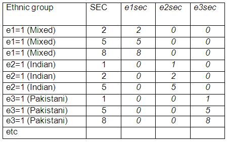
Is it reasonable to assume that ethnic group differences in attainment are the same at all levels of SEC? We mentioned above that there is an emerging literature that suggests this may not be the case. One way to allow for different slopes in the relationship between SEC and attainment for different ethnic groups is to include extra variables in the model that represent the interactions between SEC and ethnic group.

For the purpose of this first example we treat SEC as a continuous variable, as we did in Models 1-3 (Pages 3.4 to 3.8). We want to create additional explanatory variables that will represent the effect of SEC within each ethnic group. We do this simply by multiplying each of our ethnic group dummy variables by SEC. The table below (Figure 3.11.1) shows the computed values for some selected cases. e1sec will be a separate variable containing the SEC values only for cases where ethnicity =1 (Mixed heritage students); e2sec will be a separate variable contain the SEC values only for cases where ethnicity =2 (Indian students) and so on. Remember there has to be an omitted category against which these dummy variables are contrasted and this is White British students.

Figure 3.11.1: Table showing examples of new interaction variables

The inclusion of the terms e1sec to e7sec, called the interaction between ethnic group and SEC, allows for the relationship between SEC and attainment to vary for different ethnic groups. If these interaction terms are significant we say there is an interaction effect.

We have created these variables for you in the MLR LSYPE 15000 but if you like you can do it yourself using the compute menu (See Module 1) or by using the following syntax: Creating ethnicity by SEC interaction terms .

Now we add the seven variables e1sec to e7sec to our model. Go to the main regression menu again and add e1sec, e2sec, e3sec, e4sec, e5sec, e6sec, e7sec, sec, gender, and e1- e7. As always, ks3stand is our Dependent variable. Before moving on select the SAVE submenu and place a tick in the unstandardised predicted values box. SPSS will save the predicted values for each case and, as this is the second time we have requested predicted values, will name the new variable PRE_2. These predicted values will be useful later in plotting the interaction effects. Click OK to run the regression.

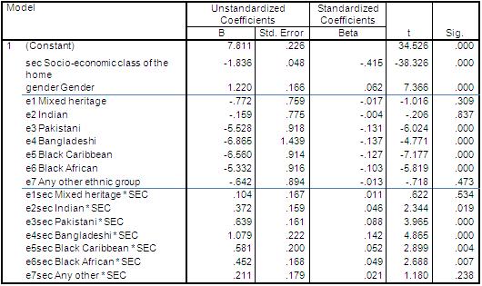
The coefficients table from the SPSS regression output is shown below.

Figure 3.11.2: Coefficients for Model 5

How do we interpret the output? As before the intercept term (Constant) refers to the predicted values for the reference or base category, which is where SEC=0, gender=0 (boy) and ethnicity=0 (White British). However the coefficient for SEC now represents the effect of SEC for the reference group only (White British students). For White British students, attainment drops by 1.836 standard score points for every unit increase in the value of SEC. To evaluate the effect of SEC for each ethnic group, we adjust the overall SEC coefficient by combining it with the relevant ethnic*sec interaction term. Thus the slope of SEC for Black Caribbean students is -1.836 + .581= -1.26, significantly less steep than the slope for White British students. This is indicated by the significant p value for the Black Caribbean * SEC interaction term (p<.000).

A good way of interpreting this data is to calculate what the predicted age 14 standard scores are from the model:

Predicted age 14 score for male White British students when SEC=5 (Lower supervisory):

Ŷ = intercept + (5 *SEC coefficient)

Ŷ = 7.81 + (5*-1.836) =-1.37

As gender=0 (male) and ethnic group=0 (White British) there is no contribution from these terms.

Predicted age 14 score for male Black Caribbean students when SEC=5 (lower supervisory).

Ŷ = intercept + (coeff. for Black Caribbean) + (5 * SEC coefficient) + (5 * Black Caribbean by SEC interaction)

Ŷ = 7.81 + -6.56 + (5*-1.836) + (5 * .581) = - 5.02

As before we can get SPSS to plot the full set of predicted values for all ethnic group and SEC combinations using the predicted values from the model that we created earlier (by default the variable was named PRE_2). Again we will plot only the values for boys since the pattern for girls is identical, except that all predicted values are 1.22 score points higher.

The syntax below temporarily filters girls out of the analysis AND draws a line graph: Creating a line graph for predicted Age 14 achievement by ethnic group and SEC for girls only . The graph is shown in Figure 3.11.4. For reference the regression lines from the model without interactions is shown in Figure 3.11.3.

Figure 3.11.3: Regression lines between ethnic group, SEC and attainment without interactions between ethnic group and SEC.

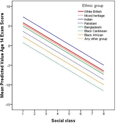
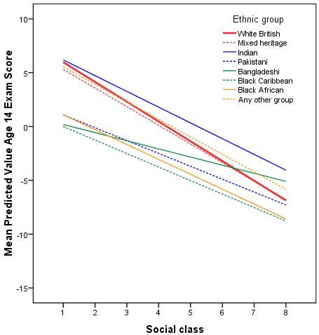
Figure 3.11.4: Regression lines between ethnic group, SEC and attainment with interactions between ethnic group and SEC.

These interaction effects between ethnic groups and SEC are highly statistically significant, particularly for the Pakistani, Bangladeshi, Black Caribbean and Black African groups. We can see this from the sig values for the interaction terms which show p<.000 for Pakistani and Bangladeshi and p<.01 for the Black Caribbean and Black African groups. They are also quite large as can be seen in Figure 3.11.4. Note here that the lines are no longer parallel because we have allowed for different slopes in our regression model. Thus the slope for White British students is significantly steeper than for most ethnic minority groups, indicating the difference in attainment between students from high SEC and low SEC homes is particularly pronounced for White British students. Looking at the predicted values we see that the differences between ethnic groups from lower SEC homes are much smaller than the differences among high SEC homes. Rather than a constant difference between White British and Black Caribbean students of 4.25 score points at every SEC value, as indicated by model 3 without the interaction terms, the difference is actually 6.0 points at SEC=1 (Higher managerial and professional homes) , 3.7 points at SEC=5 (lower supervisory) and only 1.9 points at SEC=8 (long term unemployed). There are clear interaction effects.

Have we improved the fit of our model?

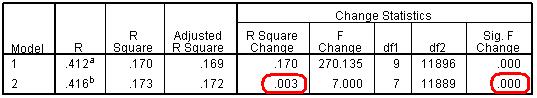
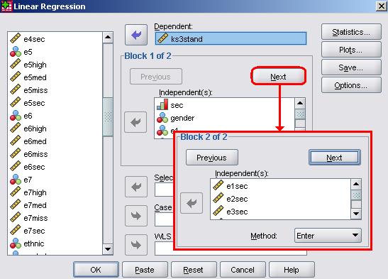
The inclusion of the interaction terms does not at first glance appear to have substantially improved the overall fit of the model; the r² has only risen from 17.0% to 17.3% (Figure 2.11.5). You might ask therefore whether the cost in added complexity caused by adding seven new interaction variables to the model was justified. While we do not appear to have explained a lot of additional variance in age 14 standard score, we can test the significance of the increase in r² by re-running our regression analysis with a few changes.

(a) On the main regression menu add the explanatory variables in two ‘blocks’. The first (Block 1) is entered as normal and should include only SEC, gender and the ethnic dummy variables (e1 – e7). This is the ‘main effects’ model. Click the Next button (shown below) to switch to a blank window and enter the variables for the second block. In this second window (Block 2) add the interaction terms which we created (e1sec – e7sec). This is the ‘interaction’ model. Note that the variables you included in Block 1 are automatically included in the interaction model. Including a second block simply means adding new variables to the model specified in the first block.

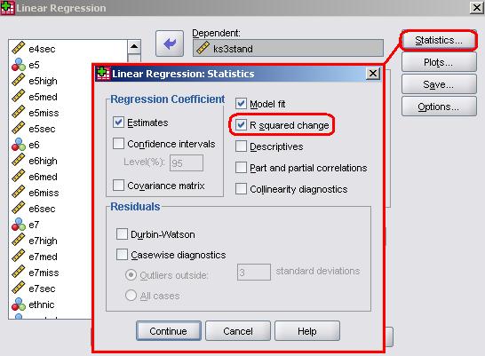
(a) Before moving on go to the Statistics sub-menu (one of the buttons on the right of the main regression menu) and check the box marked ‘R squared change’. This essentially asks SPSS to directly compare the predictive power (r²) of each model and to test if the difference between the two is statistically significant. This way we can directly test whether adding the interaction effect terms improves our model.

When you are happy with the setup, click OK to run the analysis. As an alternative method for re-running the analysis you can use the following syntax: Comparing the main effects only and interaction effects versions of Model 5 .

We get the following output under Model Summary.

Figure 3.11.5: Model summary and change statistics for Model 5

We are interested here in the columns headed ‘Change Statistics’ and specifically in the second row which compares Block 2 (the interaction model) against Block 1 (the main effects model). We can see that the increase in r² for the interaction model, while small at 0.3%, is highly statistically significant (‘Sig. F Change’, p<.000). So while the increase in overall r² is small the model with interactions gives a significantly better fit to the data than we get if the interactions are not included. In short our interaction model is a much more precise and accurate summary of the pattern of mean scores across our different explanatory variables. However the relatively low r² at 17.3% indicates that there is considerable variation in attainment between students within each category of the explanatory variables. Thus predictions of the attainment of any individual student based simply on knowledge of their SEC, ethnicity and gender, will have a large degree of imprecision. We will see later how adding further explanatory variables (such as prior attainment at age 11, Page 3.13) can substantially improve the r² for the model.

Navigation

Home
Modules
Site Guide
Module 3 Contents
Resources