Interactions between two nominal variables

The above process is relatively easy to compute (yes, I’m afraid it will get a little harder below!) but has the same problem of data loss we identified earlier. The 2941 cases that have no valid value for SEC are excluded from the model. As before we can avoid this data loss if we transform SEC to a set of dummy variables and explicitly include missing values as an additional dummy variable. This has the advantages outlined on Page 3.8. However if we keep the full eight SEC categories this would lead to a very large number of interaction terms: 7 ethnic group dummies * 8 SEC dummies (including the dummy variable for missing cases) = 56 separate interaction terms! This is substantially higher than the seven new variables we included when we treated SEC as a continuous variable on Page 3.11. Needless to say this analysing this would be a painful experience... In the interest of a parsimonious model it is unhelpful to add so many additional variables. One way to make the interactions more manageable is to ‘collapse’ the SEC variable into a smaller number of values by combining some categories.

Step 1: Collapse SEC to three levels

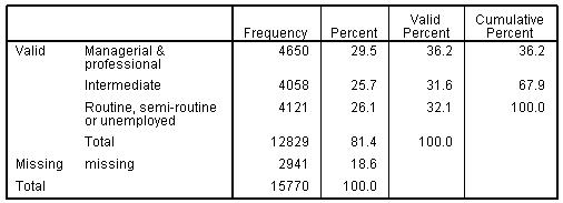
The Office for National Statistics socio-economic class (NS-SEC) coding system was used in this study. The system includes criteria for identifying 8, 5 or 3 class versions of SEC (see Resources page). To simplify the structure we recode SEC from the eight to the three class version, which combines higher and lower managerial and professional (class 1 and 2), intermediate, small employers and lower supervisory (classes 3 to 5) and semi-routine, routine and unemployed groups (classes 6 to 8). We will also create a new category for those with missing values for SEC.

All of the variables and interaction terms over the rest of this page have already been created for you in the MLR LSYPE 15000 , so you do not need to create them yourself. However, if you would like to follow the process exactly then feel free! You can either use the Recode menu (see Foundation Module) or you can run the following syntax (which will also produce a frequency table for the new variables) to create the required 3 item SEC variable: Recoding the SEC variable .

The new variable looks like this:

Figure 3.12.1: Frequencies for collapsed SEC variable

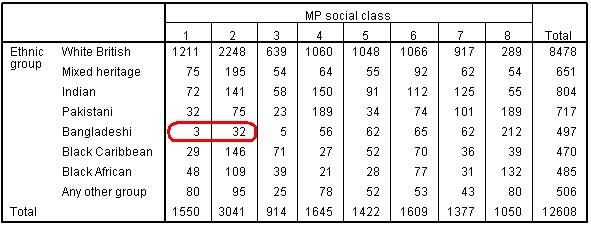
We can then calculate dummy variables for the collapsed variable, taking category 3 (low SEC) as the base or reference category. The dummy variables are already in the dataset and we have already shown you how to create dummy variables on Page 3.7, however we have included the syntax if you are interested: Creating dummy variables for SEC short .

We should note that collapsing a variable is not only useful if we want to test interactions, it is most often necessary where the number of cases in a cell is particularly low. Figure 3.12.2 shows the Crosstabulation of SEC and ethnic group. We can see there were only three Bangladeshi students in SEC class 1. By combining SEC classes 1 and 2 we increase the number of Bangladeshi students in the high SEC cell to 35. This is still relatively low compared to other ethnic groups, but will provide a more robust estimate than previously.

Figure 3.12.2: Crosstabulation of SEC by ethnic group

Step 2: Create the interaction terms

As before to create the interaction terms we simply multiply each ethnic dummy variable by the relevant SEC dummy variable. Again, we have done this for you in the MLR LSYPE 15000 dataset but if you want to do it yourself you can use the Compute option (see Foundation Module) or the following syntax: Creating ethnicity by SEC short interaction terms .

Step 3: Add the interaction terms to the model

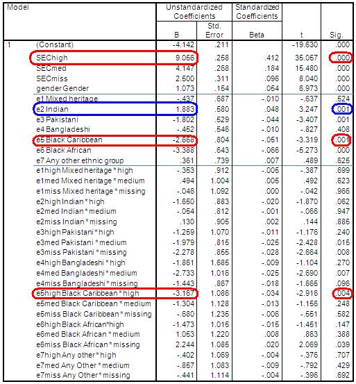
Now we can see the relationship between ethnic group, SEC and attainment using the full sample of students. Run the regression analysis including all main and interaction variables: ks3stand (Dependent), SEChigh, SECmed, SECmiss, gender, e1-e7 and all interaction terms (e.g. e1high, e1med, e1miss, e2high, e2med, e2miss, etc. Twenty-one terms in total). Remember to request predicted values from the SAVE submenu (which will be saved by default to the variable PRE_3 because this is the third time we have asked SPSS to save predicted values). Figure 3.12.3 shows the coefficient output.

Figure 3.12.3: Regression coefficients output for Model 6 

The output initially might look a little overwhelming as there are a considerable number of variables included, but this is still small compared to many models! We’re not sure if that is reassuring or not... The good thing is that the interpretation of the output is substantially the same as we saw on Page 3.11.

• The constant coefficient gives the intercept for our reference group, which is White British, boys from low SEC homes.
• The SEChigh and SECmedium coefficients are directly interpretable as the ‘boost’ to attainment for White British pupils associated with residing in medium and high SEC homes. There is a strong boost for Medium SEC (4.2 score points) and particularly for high SEC homes (9.1 score points).
• The ethnic coefficients represent the difference in attainment between each ethnic group and White British students in the reference group (low SEC homes). We see for example that Black Caribbean low SEC students on average score about 2.7 points lower than their White British low SEC peers. In contrast Indian students score about 1.9 points higher than their low SEC White British peers. Both effects are highly statistically significant (p<.001).
• The ethnic * SEC interaction terms show how the boosts associated with medium and high SEC homes vary by ethnic group. Take for example Black Caribbean students from high SEC homes. The boost associated with high SEC homes for White British students is about 9.1 points, but for Black Caribbean students it is lower, 9.056 + (-3.167) = 5.9 score points.

As before a good way of interpreting this data is to calculate what the predicted age 14 standard scores are from the model.

Predicted age 14 score for White British boys from high SEC homes:

As White British boys are the reference group this value will be calculated from just two terms: intercept + high SEC coeff.

Ŷ = -4.142 + 9.056 = 4.914

Predicted age 14 score for Black Caribbean boys from high SEC homes:

This will be calculated from: intercept + Black Caribbean coeff. + high SEC coefficient + Black Caribbean*High interaction coeff.

Ŷ = -4.142 + -2.668 + 9.056 + -3.167 = -.921

Note that gender is just modelled as a main effect (it has not been allowed to interact with SEC or ethnic group), so you would just add 1.073 to get the predicted values for girls from any ethnic or SEC group. Again we can plot the predicted value that we saved earlier when we specified the regression model (the values were saved as the variable PRE_3).

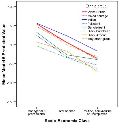
Figure 3.12.4: Predicted values for attainment at age 14 including interactions between ethnic group and SEC (Both coded as dummy variables)

There are significant interactions between the Pakistani and Bangladeshi groups and medium SEC (p=.015 and p=.007 respectively) and between Black Caribbean and high SEC (p=.004). The effects are not only statistically significant they are also quite large, as can be seen in Figure 3.12.4. Note here that the regression lines are no longer parallel because we have allowed for different slopes in our regression model. The slope for White British students is significantly steeper than for most ethnic minority groups indicating the differences between high SEC and low SEC homes is particularly pronounced for White British students. Looking at the coefficients in Figure 3.12.3 we see that the differences between ethnic groups from lower SEC homes are much smaller than the differences among high SEC homes. Note that the significance tests for the ethnic group coefficients in the SPSS output are for ethnic differences in the reference group of low SEC homes. If we want to test the significance of the ethnic group differences in high SEC homes we can just change our reference group to high SEC. Similarly if we want to test the significance of the ethnic difference at medium SEC we could change reference group to Medium SEC.

Have we improved the fit of our model?

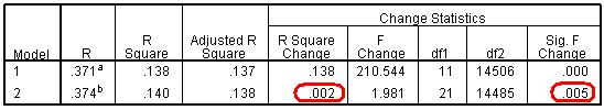
Again we can test whether we have significantly improved the r² by entering the variables in two blocks and calculating the r² change (see Page 3.11). Block 1 should include the dummy variables for SECshort, gender and ethnic group (the ‘main effects’ model), while the interaction terms should be added in Block 2 (the ‘interaction’ model).

Figure 3.12.5: Model summary and change statistics for Model 6

In Figure 3.12.5, which we received as part of our regression output, we are interested here in the columns headed ‘Change Statistics’ and specifically in the second row which compares Block 2 (the interaction model) against Block 1 (the main effects model). We can see that the increase in r² for the interaction model, while small at 0.2%, is highly statistically significant (p = .005). So while the increase in overall r² is small, the model with interactions gives a significantly better fit to the data than we get if the interactions are not included.

Navigation

Home
Modules
Site Guide
Module 3 Contents
Resources