The multiple regression model

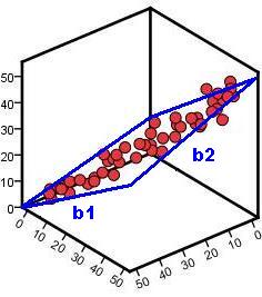
The simple linear regression model is based on a straight line which has the formula Ŷ = a + bX (where a is the intercept and b is the gradient). You'll be relieved to hear that multiple linear regression also uses a linear model that can be formulated in a very similar way! Though it can be hard to visualise a linear model with two explanatory variables we've had a go at showing you what it may look like by adding a 'plane' on the 3D scatterplot below (Figure 3.2.1). Roughly speaking, this plane models the relationship between the variables.

Figure 3.2.1: A multiple regression plane

The plane still has an intercept. This is the value of the outcome when both explanatory variables have values of zero. However there are now two gradients, one for each of the explanatory variables (b₁ on the x-axis and b₂ on the z-axis). Note that these gradients are the regression coefficients (B in the SPSS output) which tell you how much change in the outcome (Y) is predicted by a unit change in that explanatory variable. All we have to do to incorporate these extra explanatory variables in to our model is add them into the linear equation:

Ŷ = a + b₁x₁ + b₂x₂

As before, if you have calculated the value of the intercept and the two b-values you can use the model to predict the outcome Ŷ (pronounced “Y Hat” and used to identify the predicted value of Y for each case as distinct from the actual value of Y for the case) for any values of the explanatory variables (x₁ and x₂). Note that it is very difficult to visualize a scatterplot with more than two explanatory variables (it involves picturing four or more dimensions - something that sounds a bit 'Twilight Zone' to us and causes our poor brains to shut down...) but the same principle applies. You simply add a new b value (regression coefficient) for each additional explanatory variable:

Ŷ = a + b₁x₁ + b₂x₂ + b₃x₃ + ... + b_nx_n

Potentially you can include as many variables as you like in a multiple regression but realistically it depends on the design of your study and the characteristics of your sample.

Multiple R and R²

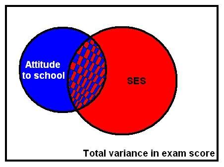
For simple linear regression it was important to look at the correlation between the outcome and explanatory variable (Pearson's r) and the r² (the coefficient of determination) to ascertain how much of the variation in the outcome could be explained by the explanatory variable. Similar statistics can be calculated to describe multiple regression models.

Multiple r is the equivalent of Pearson’s r though rather than representing the magnitude and direction of a relationship between two variables it shows the strength of the relationship between the outcome variable and the values predicted by the model as a whole. This tells us how well the model predicts the outcome (sometimes researchers say how well the model fits the data). A multiple r of 1 means a perfect fit while a multiple r of 0 means the model is very poor at predicting the outcome.

The r² can be interpreted in the exact same way as for simple linear regression: it represents the amount of variation in the outcome that can be explained by the model, although now the model will include multiple explanatory variables rather than just one. The diagram below (Figures 3.2.2 - lovingly prepared on 'MS Paint') might help you to visualize r². Imagine the variance in the outcome variable 'Exam Grade' is represented by the whole square and 'SES' (socio-economic status) and 'Attitude to School' are explanatory variables, with the circles representing the variance in exam grade that can be explained or accounted for by each.

Figure 3.2.2: SES and Attitude to School predicting Exam Grade

In Figure 3.2.2 the square represents the total variation in exam score in our sample. The red circle represents the variance in exam score that can be predicted (we might say explained) by SES. Now we add a further variable, the blue circle - attitude to school. This variable also explains a large proportion of the variance in exam score. Because attitude to school and SES are themselves related, some of the variance in exam score that can be explained by attitude is already explained by SES (hatched red and blue area). However, attitude can also explain some unique variance in exam score that was not explained by SES. The red, blue and hatched areas combined represent r², the total variance in exam score explained by the model. This is greater than would be accounted for by using either SES or attitude to school on its own.

Methods of variable selection

When creating a model with more than one explanatory variable a couple of complications arise. Firstly, we may be unsure about which variables to include in the model. We want to create a model which is detailed and accounts for as much of the variance in the outcome variable as possible but, for the sake of parsimony, we do not want to throw everything in to the model. We want our model to be elegant, including only the relevant variables. The best way to select which variables to include in a model is to refer to previous research. Relevant empirical and theoretical work will give you a good idea about which variables to include and which are irrelevant.

Another problem is correlation between explanatory variables. When there is correlation between two explanatory variables it can be unclear how much of the variance in the outcome is being explained by each. For example, the hatched area in Figure 3.2.2 represents the variance in exam score which is shared by both SES and attitude to school. It is difficult to ascertain which variable is foremost in accounting for this shared variance because the two explanatory variables are themselves correlated. This becomes even more complicated as you add more explanatory variables to the model!

It is possible to adjust a multiple regression model to account for this issue. If the model is created in steps we can better estimate which of the variables predicts the largest change in the outcome. Changes in r² can be observed after each step to find out how much the predictive power of the model improves after each new explanatory variable is added. This means a new explanatory variable is added to the model only if it explains some unique variance in the outcome that is not accounted for by variables already in the model (for example, the blue or red section in Figure 3.2.2).

SPSS allows you to alter how variables are entered and also provides options which allow the computer to sort out the entry process for you. The controls for this are shown below, but we'll go into the overall process of doing a multiple regression analysis in more detail over the coming pages. For now it is worth examining what these different methods of variable selection are.

Some of this may sound confusing. Don't worry too much if you don't get it straight away - it will become clearer when you start running your own multiple regression analyses. The main thing is that you have some understanding about what each entry method does.

Navigation

Home
Modules
Site Guide
Module 3 Contents
Resources