Using Statistical Regression Methods in Education Research

1.7 SPSS: Creating and Manipulating Variables
|
It is important that you know how to add and edit variables into your dataset. This page will talk you through the basics of altering your variables, computing new ones, transforming existing ones and will introduce you to syntax: a computer language that can make the whole process much quicker. If you would prefer a more detailed introduction you can look at the Economic and Social Data Service SPSS Guide, Chapter 5 (see Resources
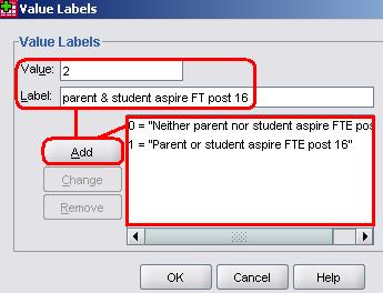
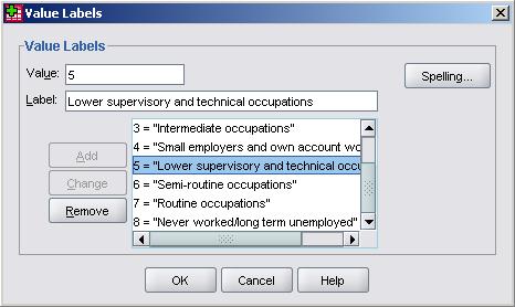
We briefly introduced the Variable View on Page 1.4 Each variable in your dataset is entered on a row in the Variable View and each column represents a certain setting or property that you can adjust for each variable in the corresponding cell. There are 10 settings: Name: This is the name which SPSS identifies the variable by. It needs to be short and can’t contain any spaces or special characters. This inevitably results in variable names that make no sense to anyone but the researcher! Type: This is almost always set to numeric. You can specify that the data is entered as words (string) or in dates if you have a specific purpose in mind... but we have never used anything but numeric! Remember that even categorical variables are coded numerically. Width: Another option we don’t really use. This allows you to restrict the number of digits that can be typed into a cell for that variable (e.g. you may only want values with two significant figures – a range of -99 to 99). Decimals: Similar to Width, this allows you to reduce the number of decimal places that are displayed. This can make certain variables easier to interpret. Nobody likes values like 0.8359415247... 0.84 is much easier on the eye and in most cases just as meaningful. Label: This is just a typed description of the variable, but it is actually very important! The Name section is very restrictive but here you can give a detailed and accurate sentence about your variable. It is very easy to forget what exactly a variable represents or how it was calculated and in such situations good labelling is crucial! Values: This is another important one as it allows you to code your ordinal and nominal variables numerically. For example you will need to assign numeric values for gender (0 = boys, 1 = girls) and ethnicity (0 = White British, 1 = Mixed Heritage, 2 = Indian, etc.) so that you can analyse them statistically. Clicking on the cell for the relevant variable will summon a pop-up menu like the one shown below.
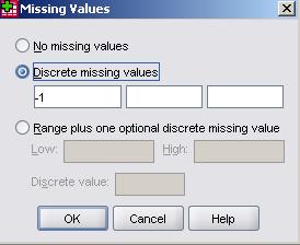
This menu allows you to assign a value to each category (level) of your variable. Simply type the value and label you want in the relevant boxes at the top of the menu and then click Add to place them in the main window. You can also Change or Remove the value labels you have already placed in the box. When you are satisfied with the list of value labels you have created click OK to finalise them. You can edit this at any time. Missing: This setting can also be very important as it allows you to tell SPSS how to identify cases where a value is missing. This might sound silly at first – surely SPSS can assign a value as missing when a value is well... not there? Actually there are lots of different types of missing value to consider and sometimes you will want to include missing cases within your analysis (Extension B
You can type in up to three individual values (or a range of values) which you wish to be coded as missing and treated as such during analysis. By allowing for multiple missing values you can make distinctions between types of missing data (e.g. N/A, Do not know, left blank) which can be useful. You can give these values labels in the normal way using the Values setting.
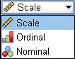
Columns: This option simply dictates how wide the column for each variable is in the Data View. It makes no difference to the actual analysis it just gives you the option of hiding or emphasising certain variables which might be useful when you are looking at your data. We rarely use this! Align: This is another aesthetic option which we don’t usually alter. It allows you to align values to the left, right or centre of their cell. Measure: This is where you define what type of data the variable is represented by. We discuss different types of data in detail on Page 1.3
Getting the type of data right is quite important as it can influence your output in a number of ways and prevent you from performing important analyses. This was a rather quick tour of the variable view but hopefully you know how to enter your variables and adjust or edit their properties. As we said, it is crucial that time is taken to get this right – you are essentially setting the structure of your dataset and therefore all subsequent analyses! Now you know how to alter the properties of existing variables we can move on to show you how to compute new ones.
Sometimes you may need to calculate a new variable based on raw data from other variables or you may need to transform data from an existing variable into a more meaningful form. Examples of this include:
For example, say we were looking at our LSYPE data and are interested in whether the parent and the student BOTH aspired to continue in full time education after the age of 16 (e.g. they wanted to go to college or university). These are two different variables but we could combine them. You would simply compute a new variable that adds all the values of the other two together for each participant.
There are occasions when you will want to reduce the number of categories in an ordinal or nominal variable by combining (‘collapsing’) them. This may be because you want to perform a certain type of analysis. We’ll show you how to do this later so don’t worry about this now! However, note that dummy variables are often a key part of regression so learning how to set them up is very important.
Again, this is not something to worry about yet... but it is an important issue that will require familiarity with the recoding process.
It may be that you want to make smaller changes to a variable to make it easier to analyse or interpret. For example, you may want to round values to one decimal place (Extension A We’ll show you the procedure for these first two examples using the LSYPE dataset, why not follow us through using LSYPE 15,000
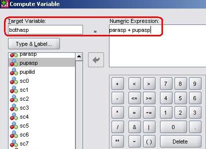
We use the Compute function to create totally new variables. For this example let’s create a new variable which combines the two existing questions in the LSYPE dataset: 1) Whether or not the parent wants their child to go to full-time education after the age of 16 (the variable named parasp in SPSS, 0 = no; 1= yes). 2) Whether or not the student themselves want to go into full-time education post-16 (pupasp; 0 = no, 1= yes). The new variable will provide us with a notion of the general educational aspirations of boththe parents and the student themselves. We will therefore give it the shortened name in SPSS of ‘bothasp’. Let’s create this new variable using the menus: Transform > Compute. The menu below will appear, featuring the calculator like buttons we saw when we were using the If menu (Page 1.4
The box marked Target Variable is for the name of the variable you wish to create so in this case we type ‘bothasp’ here. We now need to tell SPSS how to calculate the new variable in the Numeric Expression box, using the list of variables on the left and the keypad on the bottom right. Move parasp from the list on the left into the Numeric Expressionbox using the arrow button, input a ‘+’sign using the keypad, and then add pupasp. Click OK to create your new variable... If you switch to the Variable View on the main screen you will see that bothasp has appeared at the bottom.Before you begin to use it as part of your analysis remember that you will need to define its properties. It is a nominal variable not a scale variable (which is what SPSS sets as the default) and you will need to give it a label. You will also need to define Missing values of -1 and -2 and define the Values as shown:
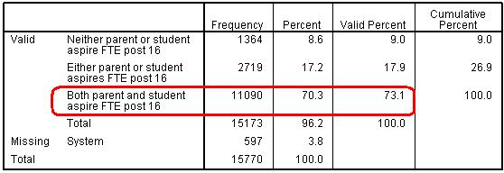
It is worth checking that the new variable has been created correctly. To do this we can run a frequency table of our new variable (bothasp) and compare it to a crosstabulation of the two original variables (parasp and pupasp). See Page 1.6 Figure 1.7.1: Frequency table for single variable Full-Time Education Aspiration
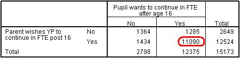
Figure 1.7.2 show a crosstabulation of the original aspiration variables. If you look at the cell where the response to both variables was ‘yes’ you will see the value of 11090, which is the same value as saw when looking at the frequency of responses for the bothasp variable. It seems the process of computing our new variable has been successful... yay! Figure 1.7.2: Crosstabulation for both Full-Time Education Aspiration variables
Once you have set up your new variable and are happy with it you can use it in your analysis!
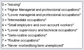
We use the recode into same variable or recode into different variableoptions when we want to alter an existing variable. Let’s look at the example of the SEC variable. There are 8 categories for this variable, and a ninth category for missing data so the values range between 0 and 9. You can check this in the Values section of the variable view:
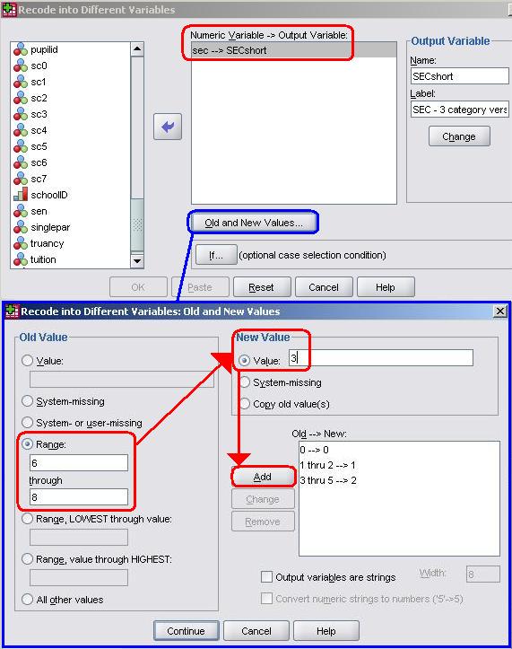
SEC is a very important variable in the social sciences and in many circumstances this fairly fine-grained variable with 9 categories is appropriate. However sometimes large numbers of categories can over complicate analysis to the point where potentially important findings can be obscured. A reasonable solution is often to combine or ‘collapse’ categories. SEC is often collapsed to a three class version, which combines higher and lower managerial and professional (categories 1 and 2), intermediate, small employers and lower supervisory (categories 3 to 5) and semi-routine, routine and unemployed groups (categories 6 to 8). These three new categories are called (1) Managerial and professional, (2) Intermediate and (3) Routine, Semi-routine or Unemployed. Let’s do this transformation using SPSS! We want to create an adapted 3 category version of the original SEC variable rather than overwriting the original so we will recode into different variables: Transform > Recode into Different Variables. You will be presented with the pop-up menu shown below, so move the SEC variable into the box marked Numeric Variable -> Output Variable. You then need to name (and Label, as you would in the Variable View) the Output Variable, which we have named SECshort (given we are essentially shortening the original SEC variable). Click the Change button to make it appear in the Numeric Variable -> Output Variable box. We now need to tell SPSS how we want the variable transformed and to do this we click on the button marked Old and New Values to open up (yet another!) pop-up menu. This one requires you to recode the old values into new ones. Moving left to right you enter the old value(s) you want to change and the new value you want to represent them (as shown). We are using the Range option because we are collapsing multiple values so that they are represented by one value (e.g. values 1 and 2 become 1, values 3, 4 and 5 become 2, etc.) You need to click on the Add button after each change of value to move it into the Old -> New window in the bottom right.
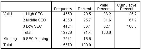
Click Continue to shut the Old and New Values window and then OK on the main recode window to create your new variable... as before, remember to check that the properties are correct and to create value labels in the Variable View. As we will see, this new SECshort variable will become useful when we turn out attention to multiple regression analysis (Module 2, Page 3.12 Let’s generate a frequency table of our new variable to check that it looks okay (See Page 1.6 Figure 1.7.3: Frequency table for 3 category SEC
We have whizzed through the process of computing and recoding variables. We wanted to give you a basic grounding as it will come in handy later but realise we have only scratched the surface. As we said, if you want to know more about these processes we recommend you use some of the materials we list on our Resources Page Let us turn our attention to another pillar of SPSS: feared by some, cherished by others, it is time to meet Syntax!
Syntax, in the context of SPSS, is basically computer language. Luckily it is quite similar to English and so is relatively easy to learn – the main difference is the use of grammar and punctuation! Basically it is a series of commands which tell SPSS what to do. Usually you enter these commands through the menus. We have already seen that this can take a while! If you know the commands and how to input them correctly then syntax can be very efficient, allowing you to repeat analyses with minor changes very quickly. Syntax is entered and operated through the Syntax Editor which is a third type of SPSS window.
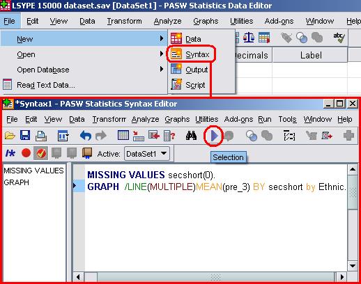
Syntax files can be saved and opened in the exact same way as any other file. If you want to open a new syntax window simply go File > New > Syntax. The image below shows you this along with an example of a Syntax window in operation.
Syntax is ‘run’, as you would run computer code. To do this you highlight the syntax you would like to use by clicking and dragging your mouse over it in the syntax window and then clicking on the highlighted ‘Run’ arrow. Whatever you have requested in your syntax, be it the creation of a new variable or a statistical analysis of existing variables – will then appear in your Data Editor and Output windows. Throughout the website we have provided SPSS Syntax files and we have occasionally provided little boxes of syntax like this one:
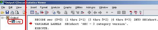
These boxes contain the syntax that you will need to paste into the Syntax Editorin order to run the related process. It may appear as though we are giving you some sort of shortcut. In a way this is true – once you have the correct syntax it is much quicker to perform processes and analyses in SPSS by using it rather than by navigating the menus. However there are other benefits too as it allows you to view more concisely the exact process that you have requested that SPSS perform. An easy way to get hold of syntax is to copy it from the Output Window. Whenever you perform an action on SPSS it is interpreted as syntax and saved to the output window. There is an example below –the syntax taken from the process of recoding the SEC variable (also shown in the above syntax alert box):
If you want to run the syntax again simply copy and paste it into the Syntax Editor. If you look at the commands you can see where you could make quick and easy edits to alter the process: VARIABLE LABELS is where the name and label are defined for example. If you wanted ‘1 thru 3’ rather than ‘1 thru 2’ to be coded as 1 you could change this easily. You may not know the precise commands for the processes but you don’t need to –run the process using the menus and examine the text to see where changes can be made. With time and perseverance you will learn these commands yourself. Attempting to teach you how to write syntax would probably be a fruitless exercise. There are hundreds of commands and our goal is to introduce you to the concept of syntax rather than throw a reference book at you. If you want such a reference book, a recommendation can be found over in our Resources |
 ?
?