Using Statistical Regression Methods in Education Research

1.10 Comparing Means
|
On Page 1.9 Field (2009), Chapter 9 (see Resources
The first thing to do is just look at the mean score on the test variable for the two groups you are interested in. Let’s see how girls and boys differ with regard to their age 14 test score (ks3stand). You can follow us through using the LSYPE 15,000 dataset
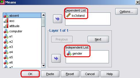
This will access a pop-up window which allows you to define your variables. Age 14 standardised exam score (ks3stand) goes in the Dependent List box because this is the variable we will be comparing our categories on. Gender goes in the Independent List because it contains the categories we wish to compare.
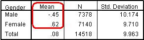
You can access the Options sub-menu to select a number of different statistics to add to your output. These are useful options and worth exploring but for now we only need the basic statistics so click OK to run the analysis. Figure 1.10.1: Basic Mean Comparison Report Output
The Case Processing Summary just tells you the number of participants used for the analysis and those who were excluded (missing) so we haven’t shown it here. Figure 1.10.1 is the Report and shows us separate mean scores on age 14 exams for boys and girls. We can see that the female mean is .62, which seems a lot higher than the male mean of -.45. When males and females are not treated separately the mean score for the students included in this analysis is .08. We can also see the number of students of each gender and the standard deviation for each gender in this table. Note that the SD for boys is slightly higher than it is for girls, demonstrating that the boy’s scores were more variable. Though there seems to be a clear difference in the means we need to check that this difference is statistically significant by providing evidence that it is unlikely to be a result of sampling variation. This is where T-tests come in.
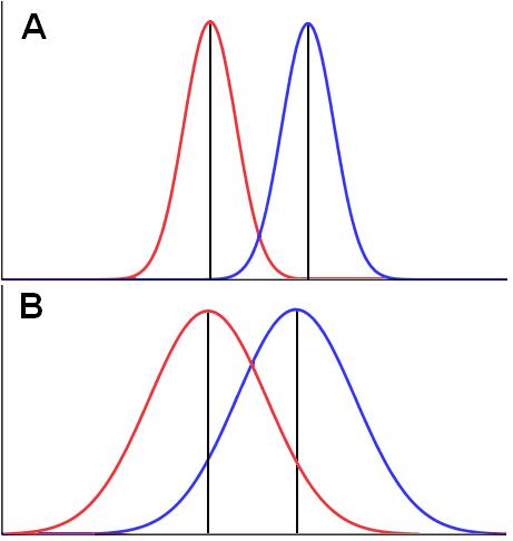
We will not get into the formula – we try to minimise our involvement with such things! Besides, there are plenty of sources available which explain the mechanics of T-tests far better than we could (don’t believe us? Check out our Resources T-tests allow you to test the statistical significance (calculate the p-value) of the difference between two means on a continuous variable. Statistical tests work on the principle that if two samples are from the same population they will have fairly similar means, but not identical since there will be random variation inherent in the sampling process. Basically we are asking if the two means are far enough apart from one another that we can be confident that they were drawn from separate populations. It is slightly more complicated than simply looking at the difference between means because we also need to consider the variance (in the form of standard deviation) within our groups along with the sample size of the two groups. Figure 1.10.2 should help you to visualise the importance of both mean and standard deviation. Imagine that boys and girls are each given their own frequency distribution of age 14 scores. The red frequency distributions represent boys and the blue ones girls, with age 14 exam score running along the horizontal x-axis. Two possible cases are outlined in the figure that illustrates the role of standard deviation. In Cases A and B the difference in male and females mean scores are the same but in Case B the standard deviations for the groups are much higher: Figure 1.10.2: The role of standard deviation when comparing means
Statistical significance is ascertained by returning to the properties of the normal distribution. As you can see in Figure 1.10.2 Case A, the mean boys score appears to be somewhere beyond two standard deviations from the mean girls score. This is outside of the 95% confidence interval and therefore unlikely to have come from the same population (p < .05). We have shown this visually but the T-test crunches the numbers to calculate it precisely. T-tests are a powerful tool but they do require you to be using something called parametric data. To be defined as parametric, your data needs to meet certain assumptions and if these are violated your conclusions can become wildly inaccurate. These assumptions are:
To complicate matters there are also three forms of t-test, each designed to deal with a specific type of research question:
Luckily the basic principles of all three tests are very similar, with only the methods tweaked to suit each type of research question. All three types are easily performed using SPSS but the most common is probably the independent samples T-test.
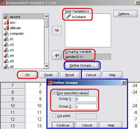
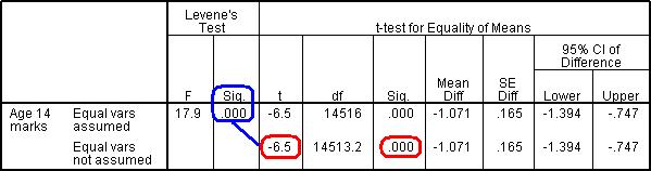
ExampleLet’s run one using our example research question from the LSYPE 15,000 Go Analyze > Compare Means > Independent Samples T Test to access the following menu: The variable we wish to compare boys and girls on is age 14 exam score (ks3stand) and needs to be placed in the Test Variable(s) window (notice how they keep changing the name of this window for different tests? Though there are good reasons for this it can get disorientating!). Our Grouping Variable is gender. Before you can proceed to run the test you will need to click on the button marked Define Groups to tell SPSS which categories within the variable you need to compare. This seems silly because we only have two categories (boys and girls) but there are times when you may want to compare two specific categories from a variable which has more than two. Also, SPSS is occasionally quite silly. Simply enter the numeric codes ‘0’ (for boys) and ‘1’ (for girls) into the Group 1 and Group 2 fields, clicking Continue when you are satisfied. Note SPSS does allow you to set a Cut point which means you can divide up scale data into two categories if you wanted to. Once all the variables are defined click OK to run the analysis. The first table contains the Group Statistics, which basically gives us the same information we saw when we ran a simple means comparison. It is the second (unwieldy long) table that we are interested in here, the Independent Samples Test (Figure 1.10.3): Figure 1.10.3: Independent samples T-test comparing age 14 exam score across gender
Note: We have cut some of the terms down slightly to fit the table on our page so it may look slightly different to your version. Let us work through this table and interpret it. The first matter to address is rather confusing but it is important. Levene’s Test tells us whether or not we are safe in our assumption that our two groups have equal variances (if you recall, this tackles point 3 of our parametric assumptions). If the test is not statistically significant then we can assume there are equal variances and use a normal T-test. However if Levene’s test is statistically significant (as is the case here) then we need to use a corrected version of the T-test... Luckily SPSS does this for you! All you need to do is use the Equal variances not assumed row of the table. Had Levene’s test been non-significant we would use the top row, Equal variances assumed. Now we know which row to examine we need only move along to the column marked ‘Sig’ to ascertain whether the differences between the boys and girls is statistically significant. We can see from the table that it is highly significant – the p-value is .000, so small it is less than 3 decimal places (p < .001)! The actual T-statistic is included which is important to report when you write up your results, though it does not need to be interpreted (it is used to calculate the p-value).The table also tells us the difference between the means (-1.071, meaning boys ‘0’ score less than girls ‘1’) and provides us with a confidence interval for this figure.
We are now confident that the difference we observed between the age 14 exam scores of males and females reflects a genuine difference between the subpopulations. However what the p-value does not tell us is the how big this difference is. Given our large sample size we could observe a very small difference in means but find that it is statistically significant. P-values are about being confident in your findings but we also need a gauge of how strong the difference is. This gauge is called the effect size. Effect size is an umbrella term for a number of statistical techniques for measuring the magnitude of an effect or the strength of a relationship. In a few cases it can be straightforward. If the dependent variable is a natural or well understood metric (e.g. GCSE grades, IQ score points) we can tell just by looking at the means – if males are scoring an average of 50% on an exam and females 55% than the effect is 5 percentage points. However, in most cases we wish to standardise our dependent variable to get a universally understood value for effect size. For T-tests this standardised effect size comes in the form of a statistic called Cohen’s d. SPSS does not calculate Cohen’s d for you but luckily it is easy to do manually. Cohen’s d is an expression of the size of any difference between groups in a standardised form and is achieved by dividing this difference by the standard deviation (SD): Cohen’s d = (Mean group A – Mean group B) / pooled SD Pooled SD = (SD group A x n group A + SD group B x n group B) / N The output statistic is a value between 0 and 1. Effect size is powerful because it can compare across many different outcomes and different studies (whatever the measure is we can calculate an effect size by dividing the difference between means by the standard deviation). Values of Cohen’s d can be interpreted as follows: Figure 1.10.4: Interpreting Effect size (Cohen’s d)
Alternatively the Cohen’s d value can be viewed as equivalent to a Z score. You can then use the normal distribution (Page 1.8, Figure 1.8.4) to indicate what percentage of one group score below the average for the other group. For example, if we found that group B had a higher mean than group A with an effect size of 0.50, this would correspond to 69.1% of group A having a score below the group B mean (but remember that 50% of group B members do as well!).
ExampleLet’s calculate the effect size for the difference in age 14 scores between males and females in the LSYPE dataset. Figure 1.10.3 tells us that the difference between the means scores for girls and boys is 1.07. We also know the standard deviations and sample sizes (n) for each group from Figure 1.10.1. All we need to do is plug these values into our formula: Pooled SD = (SD group A x n group A + SD group B x n group B) / N = (10.174 x 7378 + 9.710 x 7140) / 14518 = 9.946 Cohen’s d = (Mean group A – Mean group B) / pooled SD = 1.07/ 9.946 = .108 According to Figure 1.10.4 the value of .108 actually corresponds to a weak effect. Even though we have observed a gender difference that is highly statistically significant it is not hugely powerful. We can be confident that there is a gender difference but the difference is relatively small. Overall the results of the T-test could be written up like this: Male and female students differed significantly in their mean standardised age 14 exam score (t= -6.5, df =1453, p<.001). The male mean (mean = -.45, SD=10.2) was 1.07 standard points lower than for females (mean= .62, SD=9.7), indicating an effect size (Cohen’s d) of 0.11. Let’s now move on to look at how to handle means comparisons when there are multiple categories.
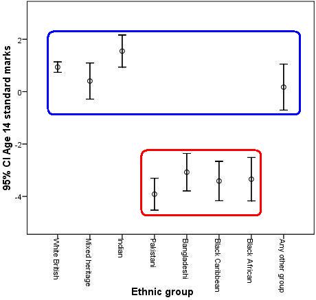
ANOVA stands for ‘Analysis of Variance’. The one-way ANOVA is very similar to the t-test but it allows you to compare means between more than two groups, providing an overall test of whether there is any significant variation in scores between these groups (producing something called an F test statistic). Basically it tests the null hypothesis that all of the group means are the same. Again, we want to only introduce the important concepts and practicalities in this module so we do not provide an explanation of how the ANOVA works (Check out our Resources We use T-tests to compare two group means but if we are interested in comparing the scores of multiple groups, we need to use a one-way ANOVA. When a variable, like gender, has two categories (male and female), there is only one comparison. However, if you have an independent variable with five categories (e.g. social science, science, art, humanities, other) then 10 comparisons, one for each pair of variables, are needed. When the overall one-way ANOVA result is significant, that does not necessarily mean that all of these comparisons (known as pair-wise comparisons) are significant. Thus, we need to find out whether all ten comparisons are significant, or just some of them. You can make such comparisons between the pairs of categories using ‘Post-hoc’ tests. These are a bit like individual T-tests which back up and elaborate upon the overall ANOVA result. Figure 1.10.5 is an adaptation of Figure 1.9.5 which illustrates the need for an ANOVA (called an ‘omnibus’ test because it provides an overall picture) to be backed up with post-hoc tests. The error bars show that there clearly is an overall effect of gender on age 14 exam scores: some ethnic groups clearly outperform others (e.g. the comparison between Indian and Pakistani students). However it is not the case that every single pair-wise comparison is statistically significant. For example, the Bangladeshi and Black Caribbean students do not appear to score much differently. We have highlighted two sets of category on the error bars below which appear to demonstrate significant differences between some pair-wise comparisons (between categories in the blue and red sets, for example White British and Pakistani) but not others (within each set, for example White British and Indian). Figure 1.10.5: Mean age 14 score by ethnicity with 95% CI Error Bars and illustration of statistically significant comparisons
Remember that when making a large number of pair-wise comparisons some are likely to be significant by chance (at the 5% level we would find 1 in 20 comparisons statistically significant just by chance). There are 18 different forms of post hoc tests (which is rather intimidating!). Your choice of post-hoc test depends on whether the group sample sizes and variances are equal and the practical significance of the results (See Field, 2009, p372-374 in our Resources for a full discussion). The following are the ones which are most frequently used: Bonferroni and Tukey are conservative tests in that they are unlikely to falsely give a significant result (type I error) but may miss a genuine difference (type II error). See Page 1.9 LSD and SNK are more liberal tests, which means that they may give a false positive result (type I error) but are unlikely to miss a genuine difference (type II error).
ExampleWe realise we have sprinted through this explanation so let’s run an example one-way ANOVA using a research question from the LSYPE 15,000 How do White British students do in exams at age 14 compared to other ethnic groups?
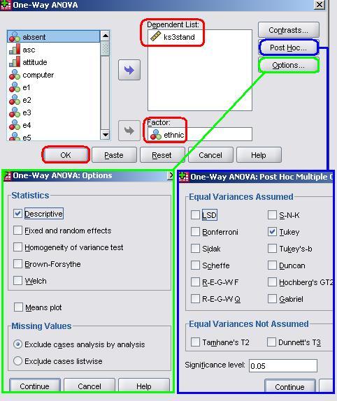
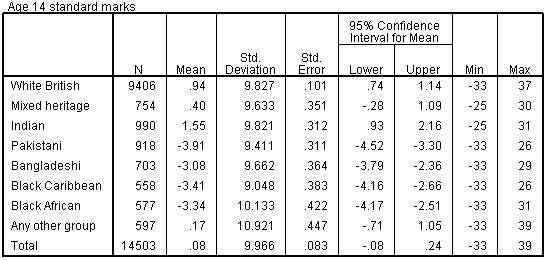
Before we continue we need to request that SPSS performs post-hoc analysis for us. Click on the button marked Post Hoc to open the relevant submenu. There is a mind boggling array of tests listed here and if you intend to perform ANOVAs in your own research we recommend you find out more about them through our Resources It is also worth checking the Options submenu. There are a number of extra statistics that you can request here, most are related to checking the parametric assumptions of your ANOVA. For now we will request only the basic Descriptive statistics to compliment our analysis. Click Continue to shut this menu and then, when you are happy with the settings click OK to run the analysis. Figure 1.10.6 shows the first table of output, the Descriptives. This is a useful initial guide as it shows us the mean scores for each ethnic group. Figure 1.10.6: Descriptives – Mean Age 14 Exam score by Ethnicity
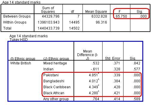
Figure 1.10.7 shows the ANOVA output along with a truncated version of the massive table marked Multiple Comparisons. We have included only the comparisons between White British students and the other groups but you will notice that the table you have is much bigger, providing pair-wise comparisons between all of the ethnic groups. The final two columns of the ANOVA table tell us that there are statistically significant differences between the age 14 scores of at least some of the different ethnic groups (F = 65.75, p < .001). This means we can reject the null hypothesis that all the means are the same. Figure 1.10.7: ANOVA Output – Age 14 Exam score by Ethnicity
The highlighted section of the Multiple Comparisons table shows the results of the post-hoc Tukey tests for the pair-wise comparisons between the White British students and the other ethnic groups. Looking down the column on the far right we can see that there are statistically significant differences with four of the seven groups. There are no significant differences between the White British students and the Mixed Heritage, Indian or ‘Other’ categories. However White British students score significantly higher than Pakistani, Bangladeshi, Black Caribbean and Black African groups (note that the stats only show that there is a difference – we had to check the means in the Descriptives table to ascertain which direction the difference was in). We would report the ANOVA results as follows: There was a significant overall difference in mean standardised age 14 exam scores between the different ethnic groups F(7, 14495) = 65.75, p<.001. Pair-wise comparisons using Tukey post-hoc tests revealed multiple statistically significant comparisons. Students from White British (Mean = .94) backgrounds scored higher than those from Pakistani (Mean =-3.91), Bangladeshi (Mean = -3.08), Black Caribbean (Mean = -3.41) and Black African (Mean = -3.34) backgrounds.
That’s it for the foundation module. Please remember that this module has given a relatively superficial coverage of some of the important topics... it is not intended to fully prepare you for regression analysis or to give you a full grounding in basic statistics. There are some excellent preparatory texts out there and we recommend you see our Resources
Now it is time to take our Quiz and perhaps work through the Exercise to consolidate your understanding before starting on the next module. Go on... Have a go! |
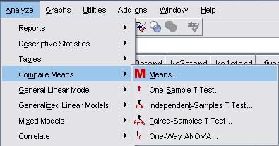
 : Analyze > Compare Means > Means.