Question 1

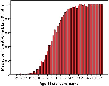
There is arguably more than one way to achieve this but we have gone for a bar graph which uses ks2stand as the category (X axis) and the mean fiveem score as the Y axis. If you have forgotten how to do this on SPSS we run through it as part of the Foundation Module.

The mean fiveem score (which varies between 0 and 1) indicates the proportion of students that achieved five or more GCSEs grades A*-C (including maths and English) at each age 11 standard score. As you can see, the mean fiveem is close to 0 or even 0 at very low age 11 scores but right up at the maximum of 1 among those with the highest age 11 scores. Note that the shape of the graph matches the ‘sigmoid’ shape for binary outcomes which we have seen throughout this module. Based on this graph there appears to be strong evidence to suggest that age 11 score is a very strong predictor of fiveem.

Question 2

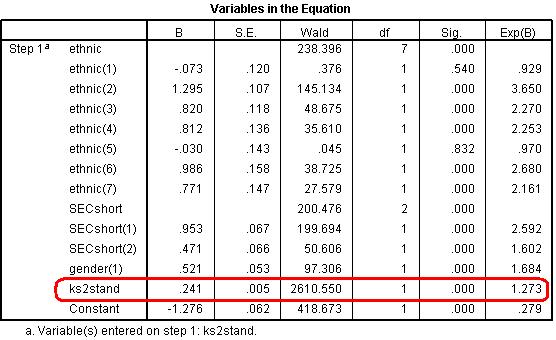
The table below shows that age 11 score is indeed a statistically significant predictor of fiveem (this can be ascertained from p<.000 in the ‘sig.’ column) even when ethnicity, SEC and gender are already in the model. The ‘Exp(B)’ column shows that the odds ratio is 1.273; meaning that a one unit change in age 11 score (an increase of 1 point) changes the odds of achieving fiveem increase by a multiplicative factor of 1.273. This is very substantial when you consider the range of age 11 scores (-24 to 39)!

See Page 4.5 if you want to review how to interpret logistic regression coefficients for continuous explanatory variables.

Question 3

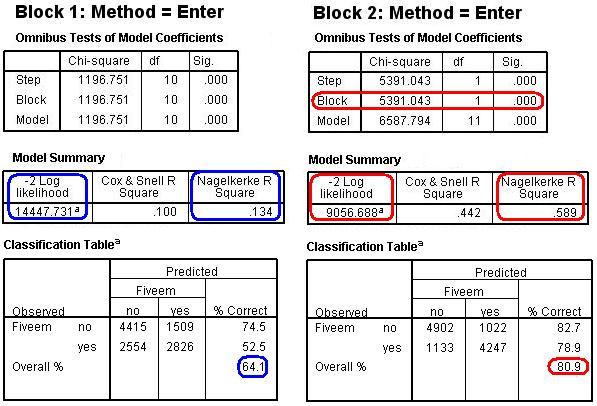
In order to explore just how much impact adding age 11 score as an explanatory variable has we re-ran the model but entered ethnic, SECshort and gender in Block 1 and ks2stand as a second block (block 2). The omnibus tests, model summary and classification tables can then be compared across these blocks to assess the impact of accounting for prior attainment at age 11. 

As we have discussed on Page 4.12, the omnibus test tells us whether or not our model is better at predicting the outcome than the ‘baseline’ model (which always predicts whichever of the two outcomes was more frequent in the data). The ‘Block’ row tells us whether the new block significantly improves the number of correct predictions compared to the previous block. Block 1 has reduced the -2LL by 1196.51 compared to the baseline model which is highly significant (p<.000). Adding age 11 score in Block 2 reduces the -2LL relative to Block 1 by a further 5391.043, which is highly statistically significant (p<.000), so the total reduction in -2LL is now 6587.794.

We can see where these reduction are calculated in the ‘Model summary’ which shows the -2LL for Block 1 is 14447 and for block 2 9056, hence the reduction in -2LL associated with adding age 11 score of 5391. More importantly the Model Summary shows us the Nagelkerke pseudo-R² is .589 (58.9% of variance explained) for block 2 compared to .134 (13.4% of variance explained) for block 1. Overall, age 11 score is clearly very important for explaining age 16 exam success!

The classification table (third table down) shows us just how much more accurately block 2 predicts the outcome compared to block 1. The model defined as block 1 correctly classifies 64.1% of cases – an improvement over the baseline model but still not great. The inclusion of ks2stand in block 2 increases the number of correct classifications substantially, to 80.9%.

 

Question 4

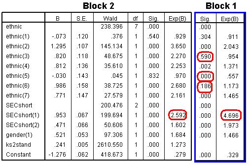
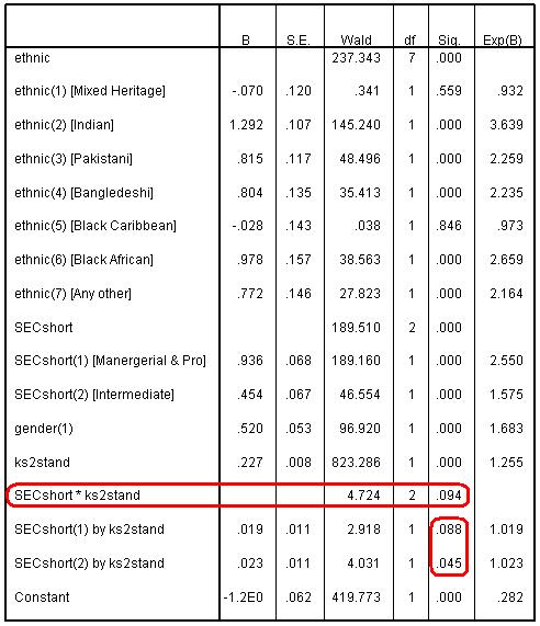
Below you will see the ‘Variables in the Equation’ table for block 2 with the ‘sig’ and Exp(B) columns from the same table for block 1. These are taken from the same SPSS output that we generated for question 3. Notice how in most cases the odds ratios [Exp(B)] are less in block 2 than they were in block 1.

For example, as highlighted, students from a managerial or professional family background [SECshort(2)] are 4.7 times more likely to achieve fiveem than those from routine, semi-routine or unemployed family backgrounds, before entering age 11 score. However, when we include age 11 score in block 2 the odds ratio reduces: those from managerial and professional homes are now 2.6 times more likely to achieve fiveem than those from the lowest SEC category. This suggests that some the difference in success rate associated with social class can be explained by prior attainment. However this is still a very sizeable difference associated with the SEC of the home, even after accounting for age 11 attainment.

Question 5

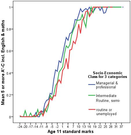
Before exploring the interaction statistically it is worth first examining the relationship by looking at a line graph (though remembering that this graph does not account for the influence of other explanatory variables such as gender and ethnicity).

As you may recall from Page 4.13, if the lines in this graph were approximately parallel we would expect there to be no interaction. The graph does not give a clear cut answer… you could argue that in the middle range of age 11 scores there is a clear ordering by SEC whereby the high SEC category has the highest pass rate and the low SEC category the lowest, but there are fluctuations, particularly at the upper and lower ends of the age 11 score range. We need to test the possibility of an interaction through the model.

Let us check the ‘Variables in the equation’ for the logistic regression model when we include a ks2stand*SECshort interaction term. This indicates that the p value associated with the overall test of interaction (SECshort*ks2stand) p=.094 is not substantial enough to reach conventional levels of statistical significance (p value is not <.05). Given that the interaction effect does not appear to be particularly pronounced (the odds ratios are relatively small for the interactions and the odds ratios for the other variables have changed very little) we would probably not include it for the sake of parsimony.

 

Question 6

As we saw on Page 4.14, cases that are having a particularly large influence on a model can be identified by requesting a statistic called Cook’s distance. If this statistic is greater than 1 for a given case, then that case may be an outlier that is powerful enough to unduly influence a model. This is usually a more significant issue when you have a small sample compared to the very large sample we have here. The table below shows the Cook’s distances produced by the interaction model we created in Question 5. We have completely removed the middle section because it is a horrendously long table. The Cook’s distances are in the left-most column and listed in numerical order. As you can see largest value (at the bottom of the table) is .05158. This is much lower than a value of 1, which would usually be cause for concern. It seems that our model has no cases that are overly influential.

Question 7

a) Is the SECshort*singlepar interaction statistically significant?

Yes, because p=.009 for the interaction term in the ‘Variables in the Equation’ table.

 

b) What is the OR for the increase in the odds of eligibility for FSM for single parent vs. dual parent families from low SEC homes?

The OR is 3.68 / 1 = 3.68. Among students from routine, semi-routine and long-term unemployed homes those from single parent families are over 3.5 times more likely to be entitled to a FSM than those from dual parent families.

 

c) What is the OR for the increase in the odds of eligibility for FSM for single parent vs. dual parent families from high SEC homes?

This OR is 0.31 / 0.05 = 6.2. Among pupils from managerial and professional homes those from single parent families are 6.2 times more likely to be entitled to a free school meal than those from dual parent families.

 

d) What is the ratio of these two ORs?

The OR for the increase in the odds of being entitled to a free school meal for single parent families from managerial homes vs. the increase for single parent families from routine homes is 6.2 / 3.68 = 1.68. So the proportionate increase in the odds of being eligible for a FSM is greater among high SEC families.

We do not have to calculate this because this is what the exponent of the SEC*Single parent interaction tells us: Exp(.52) = 1.68 (note that the figure is slightly different from the logit of .56 shown in the table due to rounding). In short the OR for an interaction between two categorical variables is the ratio of two ORs! If the two ORs are identical then the ratio of the two ORs should equal 1.0. To the extent that the two component ORs are not the same then the interaction OR will depart from 1.0.

So to conclude, while the absolute level of entitlement to a free school meal is higher among single parent families from routine homes than among single parent families from managerial homes (as we see in the graph) the increase in the odds of being entitled to a FSM associated with single parent status is proportionately greater among managerial & professional homes than among routine, semi-routine and LT unemployed homes.

Navigation

Home
Modules
Site Guide
Module 4 Contents
Resources