Using Statistical Regression Methods in Education Research

2.4 Correlation Coefficients
|
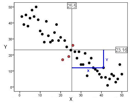
Graphing your data is essential to understanding what it is telling you. Never rush the statistics, get to know your data first! You should always examine a scatterplot of your data. However it is useful to have a numeric measure of how strong the relationship is. The Pearson r correlation coefficient is a way of describing the strength of an association in a simple numeric form. We're not going to blind you with formulae but is helpful to have some grasp of how the stats work. The basic principle is to measure how strongly two variables relate to each other, that is to what extent do they covary. We can calculate the covariance for each participant (or case/observation) by multiplying how far they are above or below the mean for variable X by how far they are above or below the mean for variable Y. The blue lines coming from the case on the scatterplot below (Figure 2.4.1) will hopefully help you to visualise this. Figure 2.4.1: Scatterplot to demonstrate the calculation of covariance The black lines across the middle represent the mean value of X (25.50) and the mean value of Y (23.16). These lines are the reference for the calculation of covariance for all of the participants. Notice how the point highlighted by blue lines is above the mean for one variable but below the mean for the other. A score below the mean creates a negative difference (approximately 10 - 23.16 = -13.6) while a score above the mean is positive (approximately 41 - 25.5 = 15.5). If an observation is above the mean on X and also above the mean on Y than the product (multiplying the differences together) will be positive. The product will also be positive if the observation is below the mean for X and below the mean for Y. The product will be negative if the observation is above the mean for X and below the mean for Y or vice versa. Only the three points highlighted in red produce positive products in this example. All of the individual products are then summed to get a total and this is divided by the product of the standard deviations of both variables in order to scale it (don't worry too much about this!). This is the correlation coefficient, Pearson's r.
The correlation coefficient tells us two key things about the association:
It is also important to use the data to find out:
Let us return to the example used on the previous page - the relationship between age 11 and age 14 exam scores. This time we will be able to produce a statistic which explains the strength and direction of the relationship we observed on our scatterplot. This example once again uses the LSYPE 15,000
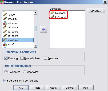
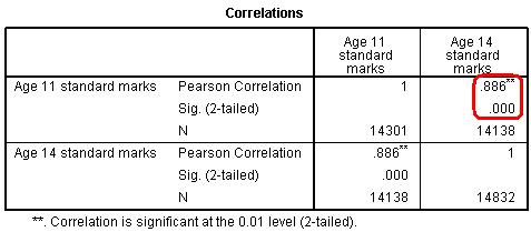
The pop-up menu (shown below) will appear. Move the two variables that you wish to examine (in this case ks2stand and ks3stand) across from the left hand list into the variables box. Note that continuous variables are preceded by a ruler icon - for Pearson's r all variables need to be continuous. The other options are fine so just click OK. SPSS will provide you with the following output (Figure 2.4.2). This correlation table could contain multiple variables which is why it appears to give you the same information twice! We've circled in red the figure for Pearson's r and below that is the level of statistical significance. Figure 2.4.2: Correlation matrix for ks2 and ks3 exam scores
As inferred from the scatterplot on the previous page, there is a positive correlation between age 11 and age 14 exam performances such that a high score in one is associated with a high score in the other. The value of .886 is strong - it means that one variable accounts for about 79% of the variance in the other (r2 = .886 x .886 = .785). The significance level of .000 means that there is a less than .0005 possibility that this difference may have occurred purely due to sampling and so it is highly likely that the relationship exists in the population as a whole.
Pearson's r is a correlation coefficient for use when variables are continuous (scale). In cases where data is ordinal the Spearman Rho rank order correlation is more appropriate. Luckily this works in a similar way to Pearson's r when using SPSS/PASW and produces output which is interpreted in the same way. If your bivariate correlation involves ordinal variables perform the procedure exactly as you would for a Pearson's correlation (Analyze > Correlate > Bivariate) but be sure to check the Spearman box in the correlation coefficients section of the pop up box and deselect the Pearson option.
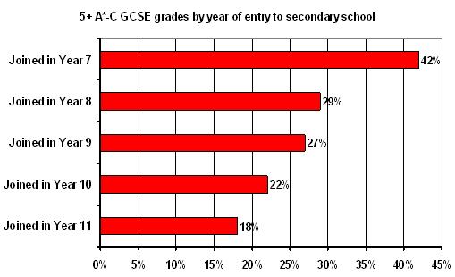
It is very important that correlation does not get confused with causation. All that a correlation shows us is that two variables are related, not that one necessarily causes the other. Consider the following example. When looking at National test results, pupils who joined their school part of the way through a key stage tend to perform at the lower end of the attainment scale than those who attended school for the whole of the key stage. The figure below (Figure 2.4.3) shows the proportion of pupils who achieve 5 or more A*-C grades at GCSE (in one region of the UK). While 42% of those who were in the same school for the whole of the secondary phase achieved this only 18% of those who joined during year 11 did so. Figure 2.4.3: Proportion of students with 5+ A*-C grades at GCSE by year they joined their school
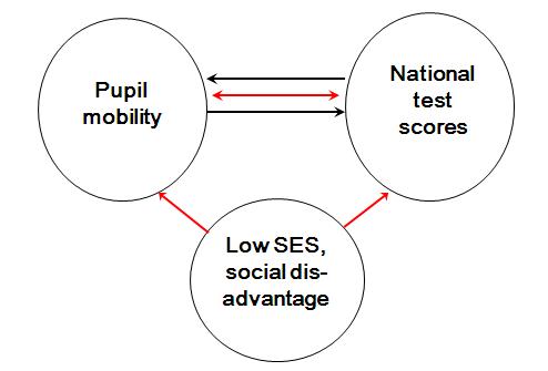
It may appear that joining a school later leads to poorer exam attainment and the later you join the more attainment declines. However we cannot necessarily infer that there is a causal relationship here. It may be reverse causality, for example where pupils with low attainment and behaviour problems are excluded from school. Or it might be that the relationship between mobility and attainment arises because both are related to a third variable, such as socio-economic disadvantage. Figure 2.4.4: Possible causal routes for the relationship between GCSE attainment and pupil mobility
This diagram (Figure 2.4.4) represents three variables but there may be hundreds involved in the relationship! We will begin to tackle issues like this more in the multiple linear regression chapter |
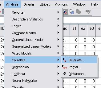
 dataset. Take the following route through SPSS: Analyze > Correlate > Bivariate (shown below).