Regression and correlation

If you are wrestling with all of this new terminology (which is very common if you're new to stats, so don't worry!) then here is some good news: Regression and correlation are actually fundamentally the same statistical procedure. The difference is essentially in what your purpose is - what you're trying to find out. In correlation we are generally looking at the strength of a relationship between two variables, X and Y, where in regression we are specifically concerned with how well we can predict Y from X.

Examples of the use of regression in education research include defining and identifying under achievement or specific learning difficulties, for example by determining whether a pupil's reading attainment (Y) is at the level that would be predicted from an IQ test (X). Another example would be screening tests, perhaps to identify children 'at risk' of later educational failure so that they may receive additional support or be involved in 'early intervention' schemes.

Calculating the regression line

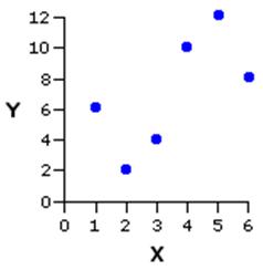
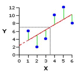
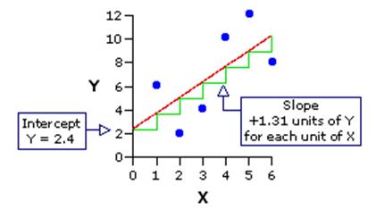
In regression it is convenient to define X as the explanatory (or predictor/independent) variable and Y as the outcome (or dependent) variable. We are concerned with determining how well X can predict Y.

It is important to know which variable is the outcome (Y) and which is the explanatory variable (X)! This may sound obvious but in education research it is not always clear - for example does greater interest in reading predict better reading skills? Possibly. But it may be that having better reading skills encourages greater interest in reading. Education research is littered with such 'chicken and egg' arguments! Make sure that you know what your hypothesis about the relationship is when you perform a regression analysis as it is fundamental to your interpretation.

Let's try and visualise how we can make a prediction using a scatterplot:

Figure 2.5.1	Figure 2.5.2

• Figure 2.5.1 plots five observations (XY pairs). We can summarise the linear relationship between X and Y best by drawing a line straight through the data points. This is called the regression line and is calculated so that it represents the relationship as accurately as possible.
• Figure 2.5.2 shows this regression line. It is the line that minimises the differences between the actual Y values and the Y value that would be predicted from the line. These differences are squared so that negative signs are removed, hence the term 'sum of squares' which you may have come across before. You do not have to worry about how to calculate the regression line - SPSS/PASW does this for you!

Figure 2.5.3

• The line has the formula Y = A + BX, where A is the intercept (the point where the line meets the Y axis, where X = 0) and B is the slope (gradient) of the line (the amount Y increases for each unit increase in X), also called the regression coefficient. Figure 2.5.3 shows that for this example the intercept (where the line meets the Y axis) is 2.4. The slope is 1.31, meaning for every unit increase in X (an increase of 1) the predicted value of Y increases by 1.31 (this value would have a negative sign if the correlation was negative).
• The regression line represents the predicted value of Y for each value of X. We can use it to generate a predicted value of Y for any given value of X using our formula, even if we don't have a specific data point that covers the value. From Figure 2.5.3 we see that an X value of 3.5 predicts a Y value of about 7.
• Of course, the model is not perfect. The vertical distance from each data point to the regression line (see Figure 2.5.2) represents the error of prediction. These errors are called residuals. We can take the average of these errors to get a measure of the average amount that the regression equation over-predicts or under-predicts the Y values. The higher the correlation, the smaller these errors (residuals), and the more accurate the predictions are likely to be.

We will have a go at using SPSS/PASW to perform a linear regression soon but first we must consider some important assumptions that need to be met for simple linear regression to be performed.

Navigation

Home
Modules
Site Guide
Module 2 Contents
Resources