Using Statistical Regression Methods in Education Research

Module 2 Exercise Answers
|
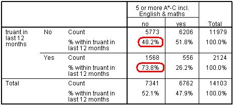
In this case we are looking for association with two nominal variables.
The best way to do this is to use a chi-square analysis. The expected crosstabulation is shown
below.
Page 2.2
Of those students who had been truant in the last year 73.8% did not achieve 5 A*-C grades at GCSE (including Maths and English). This is compared to 48.2% of students who had not been truant. It seems that those who have played truant are less likely to achieve the GCSE target. We can test how probable it is to find this association by chance when in fact there isn’t one in the population by using the Chi-square test table shown below.
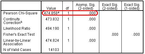
The Pearson Chi-Square confirms that the association we have spotted is statistically significant. The value of 474.858 (df = 1) has ‘Asymp Sig’ of .000, which means that p < .0005. SPSS/PASW has done it’s very best to befuddle us with a huge amount of confusingly labelled output but we have emerged victorious. Huzzah! Overall your answer to this question could look a bit like this: An association was found between whether a student had been truant (in the last 12 months) and whether they had achieved 5 or more A* - C grades at GCSE (including English and Maths), Chi-square = 474.86, df = 1, p < .0005. Examination of the cross-tabulation suggests that this association stems from those who have played truant in the last twelve months being more unlikely to achieve 5 A* - C grades at GCSE.
In this case we are looking at an association between two continuous variables and so we can explore how they correlate. The first thing to do in such situations is create a scatterplot of the data! After that we can calculate a correlation coefficient for the relationship (usually a Pearson’s coefficient). Pages 2.3 and 2.4 explain how to generate a scatterplot and how to perform a bivariate correlation if you need to refresh. You should get a scatterplot a little like the one below:
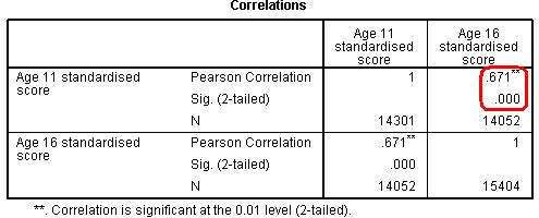
According to the ‘Pearson Correlation’ row the coefficient of .671 is strong and positive just as we may have expected based on the scatterplot. The value of .000 in the ‘Sig’ row suggests that if there was no association between these two variables the probability of obtaining a coefficient of this strength with a sample of this size would be very small, p < .0005. Your answer to this question could look like this: A strong positive correlation was found between age 11 and age 16 exam scores, r = .671, p < .0005.
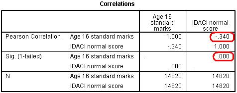
This question is the trickiest as it requires you to perform a full simple linear regression analysis! Pages 2.7 The correlation coefficient between Age 16 exam score and IDACI is negative, r = -.340 which means that as level of deprivation increases GCSE scores decrease.
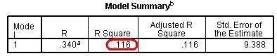
The model summary tells us how much of the variance in our outcome variable is accounted for by our predictor variable (that is how much variance does the simple linear regression model account for). The R Square column gives us this value, which is known as the coefficient of determination, r2, as .116. In other words IDACI score accounts for 12% of the variance in age 16 exam score.
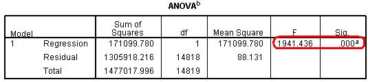
The ANOVA table tells us whether or not our simple linear regression model is better at predicting the outcome variable than simply using the mean of the outcome variable. The F-ratio of 1941.4 (see column F) is statistically significant at p < .0005 (Column: Sig= .000), suggesting that our model does improve the prediction.
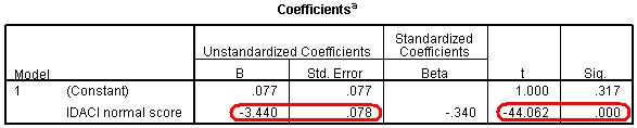
The coefficients table provides lots of information about the model. The intercept (where IDACI score = 0) is provided in the ‘B’ column for the ‘(Constant)’ row as .077 while the gradient of the regression line (the coefficient) is in the ‘B’ column of the ‘IDACI normal score’ row: -3.440. This means that for each standard deviation that the normalised IDACI score increases the predicted age 16 score decreases by 3.4 standard units. The final two columns for this row (t = -44.062, p < .0005) tell us that IDACI is a statistically significant predictor of the outcome (age 16 exam score).
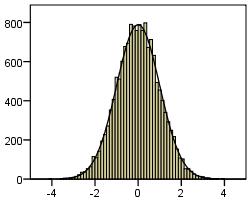
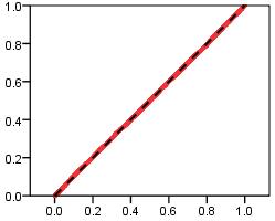
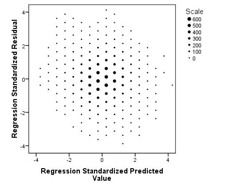
Above are miniaturised versions of the histogram and P-P plot that you should find in your output. As you can see the residuals show no major departures from the normal distribution to be overly concerned with. The above scatterplot can be used to identify homoscedasticity. Note that we have used ‘binning’ on our version so that we can make out the pattern of the data more easily. The plot seems to show a fairly random spread of residuals (as we would hope for our assumptions). Homoscedasticity does not appear to be problematic. Overall your answer to the question might look a bit like this:
|
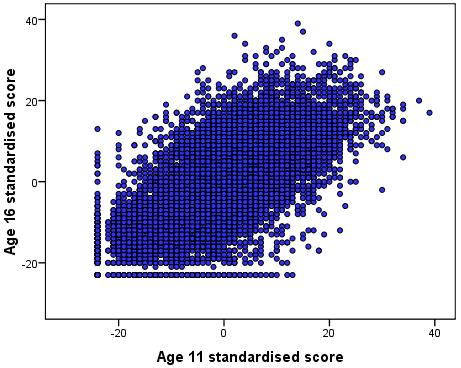 You have probably noticed how this is similar to the scatterplot for the age 11 and age 14 data. It looks as though past performance has a positive correlation with more recent performance even over this
greater timescale. Let us check this statistically with a correlation coefficient.
You have probably noticed how this is similar to the scatterplot for the age 11 and age 14 data. It looks as though past performance has a positive correlation with more recent performance even over this
greater timescale. Let us check this statistically with a correlation coefficient.