Using Statistical Regression Methods in Education Research

2.2 Association
|
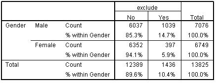
It is useful to explore the concepts of association and correlation at this stage as it will hold us in good stead when we start to tackle regression in greater detail. Correlation basically refers to statistically exploring whether the values of one variable increase or decrease systematically with the values of another. For example, you might find an association between IQ test score and exam grades such that if individuals have high IQ scores they also get good exam grades while individuals who get low scores on the IQ test do poorly in their exams. This is very useful but association cannot always be ascertained using correlation. What if there are only a few values or categories that a variable can take? For example, can gender be correlated with school type? There are only a few categories in each of these variables (e.g. male, female). Variables that are sorted into discrete categories such as these are known in SPSS/PASW as nominal variables (see our page on types of data in the prologue). When researchers want to see if two nominal variables are associated with each other they can't use correlation but they can use a crosstabulation (crosstab). The general principle of crosstabs is that the proportion of actual observations in each category may differ from what would be expected to be observed by chance in the sample (if there were no association in the population as a whole). Let's look at an example using SPSS/PASW output based on LSYPE data (Figure 2.2.1): Figure 2.2.1: Crosstabulation of gender and exclusion rate
This table shows how many males and females in the LSYPE sample were temporarily excluded in the three years before the data was collected. If there was no association between gender and exclusion you would expect the proportion of males excluded to be the same or very close to the proportion of females excluded. The % within gender for each row (each gender) displays the percentage of individuals within each cell. It appears that there is an association between gender and exclusion - 14.7% of males have been temporarily excluded compared to 5.9% of females. Though there appears to be an association we must be careful. There is bound to be some difference between males and females and we need to be sure that this difference is statistically improbable (if there was really no association) before we can say it reflects an underlying phenomenon. This is where chi-square comes in! Chi-square is a test that allows you to check whether or not an association is statistically significant.
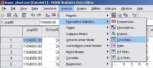
Why not follow us through this process using the LSYPE 15,000 To draw up a crosstabulation (sometimes called a contingency table) and calculate a chi-square analysis take the following route through the SPSS data editor: Analyze > Descriptive Statistics > Crosstabs
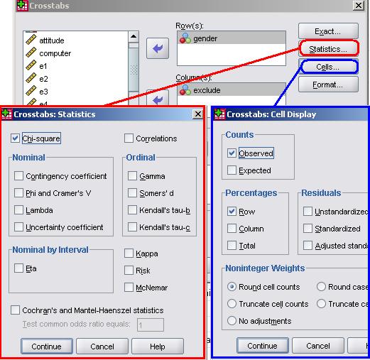
Now move the variables you wish to explore into the columns/rows boxes using the list on the left and the arrow keys. Alternatively you can just drag and drop! In order to perform the chi-square test click on the Statistics option (shown below) and check the chi-square box. There are many options here that provide alternative tests for association (including those for ordinal variables) but don't worry about those for now.
Click on continue when you're done to close the statistics pop-up. Next click on the Cells option and under percentages check the rows box. Click on continue to close the pop up and, when you're ready click OK to let SPSS weave its magic...
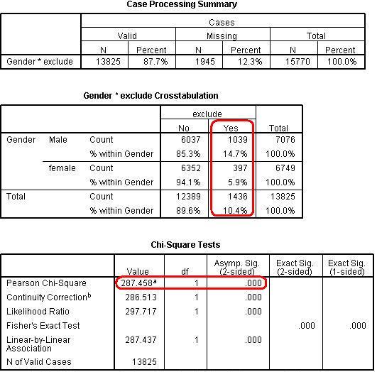
You will find that SPSS will give you an occasionally overwhelming amount of output but don't worry - we need only focus on the key bits of information. Figure 2.2.2: SPSS output for chi-square analysis
The first table of Figure 2.2.2 tells us how many cases were included in our analysis. Just below 88% of the participants were included. It is important to note that over a tenth of our participants have no data, but 88% is still a very large group - 13,825 young people! It is very common for there to be missing cases as often participants will miss out questions on the survey or give incomplete answers. Missing values are not included in the analysis. However it is important to question why certain cases may be missing when performing any statistical analysis - find out more in our missing values section, Extension B The second table is basically a reproduction of the one at the top of this page (Figure 2.2.1). The part outlined in red tells us that males were disproportionately likely to have been excluded in the past three years compared to females (14.7% of males were excluded compared to 5.9% of females). Chi-square is less accurate if there are not at least five individuals expected in each cell. This is not a problem in this example but it is always worth checking, particularly when your research involves a smaller sample size, more variables or more categories within each variable (e.g. variables such as social class or school type). The third table shows that the difference between males and females is statistically significant using the Pearson Chi-square (as marked in red). The Chi-square value of 287.5 is definitely significant at the p < .05 level (see Asymp. Sig. column). In fact the value is .000 which means that p< .0005. In other words the probability of getting a difference of this size between the observed and expected values purely by chance (if in fact there was no association between the variables) is less than 0.05% or 1 in 2,000! We can therefore be confident that there is a real difference between the exclusion rates of males and females.
Chi-square provides a good method for examining association in nominal (and sometimes ordinal) data but it cannot be used when data is continuous. For example, what if you were recording the number of pupils per school as a variable? Thousands of categories would be required! One option would be to create categories for such continuous data (e.g. 1-500, 501-1000, etc.) but this creates two difficult issues: How do you decide what constitutes a category and to what extent is the data oversimplified by such an approach? Generally where continuous data is being used a statistical correlation is a preferable approach for exploring association. Correlation is a good basis for learning regression and will be our next topic. |
 dataset. We also have a
  .
.