Using Statistical Regression Methods in Education Research

Module 1 Exercise Answers
|
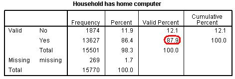
What percentage of students in the LSYPE dataset come from a household which owns a computer (computer)? By using Analyze > Descriptive Statistics > Frequencies the following table can be produced:
It shows that 87.9% of students who answered this question (the valid cases) come from a household which owns a computer.
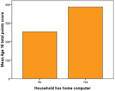
Let’s say you are interested in the relationship between achievement in exams at age 16 and computer ownership. Create a graph which compares those who own a computer to those who do not (computer) with regard to their average age 16 exam score (ks4score). A bar chart can be produced by using Graphs > Legacy Dialogs > Bar. You need to select Other Statistic (Mean) for ‘bars represent’ and choose age 16 exam score.
It seems that those from families who do own a computer have a higher mean score in age 16 examinations.
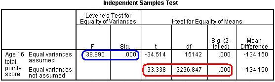
Is the difference between the average age 16 exam scores (ks4score) for those who do and do not own a computer (computer) statistically significant? The t-test can be performed using Analyze > Compare Means > Independent Samples T-test. ks4score is the test variable and computer is the grouping variable. You should get the following output:
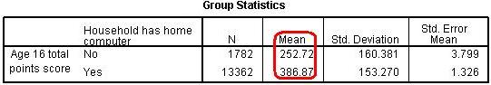
The first table displays the descriptive statistics which tells us the mean Age 16 exam score and standard deviation for each group. There appears to be a substantial difference between the groups. The second table shows the T-test itself. Note that Levene’s test is statistically significant which means we should not assume equal variances in the two groups and should use the adjusted figures in the second row (highlighted in red). The T-test shows that there is indeed a statistically significant difference between the mean age 16 exam scores of those from families with a computer compared to those from families without one (t = 33.3, df = 2237, p < .0005).
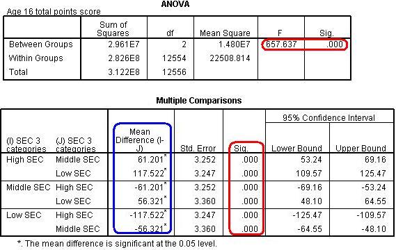
Let’s look at the relationship between social-economic class (secshort) and achievement in exams at age 16. Is there a difference between the three SEC groups (high, medium and low SEC) with regard to their average achievement in age 16 exams (ks4score)? If so which groups differ? A one way ANOVA can be performed using Analyze > Compare Means > One-Way ANOVA. We use ks4score as the dependent variable and secshort as the factor. From the ‘Post-Hoc’ submenu you should select ‘Scheffe’ in order to perform the relevant pair wise post-hoc comparisons between SEC groups. You should generate the following output:
The first thing to notice is that, according to the omnibus F-test, there is a statistically significant difference between the groups overall, F = 657.6, df = 2, 12554, < .0005. We need to look at the post-hoc analysis to explore where these differences actually are. It appears that all three SEC groups are different from one another! The mean difference column shows us the ‘High SEC’ group scores an average of 61 more points than the ‘Middle SEC’ group and 117.5 more than the ‘Low SEC’ group. The ‘Middle SEC’ group scores 56 more points on average than the ‘Low SEC’ group. As shown in the column headed ‘Sig.’ all of these differences are highly statistically significant.
Create an error bar graph which illustrates the difference between SEC groups (secshort) with regard to their average achievement in age 16 exams (ks4score). An error bar chart can be produced by using Graphs > Legacy Dialogs > Error Bar. You should be able to produce a chart which looks like this: From this chart you can see that there are clear differences between the mean age 16 exam scores for each group (the circle in the centre of each error bar), with the ‘High SEC’ group outperforming the ‘Middle SEC’ group, who in turn outperform the ‘Low SEC’ group. The error bars themselves encompass the range of scores within which we are 95% sure that the true mean in the population lies (a 95% confidence interval). The fact that the error bars do not overlap implies that the differences between groups are statistically significant (something we actually know to be true based on question 4). |