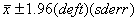
About this Resource
P|E|A|S FAQ   | home   | contact us   | index   | links and further resources   |

4. Standard Errors and Design Effects

uparrowtop

4.1 What is a standard error?

How far is my survey estimate from the ‘true’ population value?.

If we know how a survey was designed and what sample size was achieved then we can work out how far a survey estimate is likely to be from the truth about your population.

We try to design surveys so as to get unbiased answers that will not (on average) consistently differ from the truth. But even an unbiased sample (see figure below) will not always get us precisely the correct answer.

estimates picture
Figure 4.1: : Bias and precision of estimates

We measure the precision of an estimator by how far we expect it to be from the average of the estimates we might obtain from many similar surveys. Here it is represented by the average distance from the individual points to the center point of the cluster.

This average distance is the standard error of our estimate.

Precise estimates (top row) have small standard errors and imprecise ones (bottom row) have large standard errors.

Here we show not just one, but several estimates. For any real survey we would only have one estimate. But statistical theory, based on knowledge of the design, can tell us what our standard error will be.

For InfoButtonunbiased estimates the standard error becomes the average distance of our estimate from its true value, the bull’s eye in the picture. A result that holds generally for most large samples is that 95% of all unbiased estimates will lie within 2 standard errors of the true value. A range that includes 95% of all estimates is called a 95% confidence interval. Sometimes the phrase ‘margin of error’ is used for twice the standard error.

uparrow
Philosophical Aside
Just how a confidence interval is defined depends on which philosophy of statistics you subscribe to. A frequentist would say that a confidence interval is 95% certain to contain the true value, which is judged from considering all possible surveys that might have been done, only one of which you have actually carried out. A Bayesian statistician (who might want to call it a 95% credible interval) would say that it defines your belief, derived from the sample, as to where the true population value lies.

Practical matters
In practice both philosophies give us the same answers almost all of the time. The tool kit for calculating standard errors and confidence intervals tell us about the uncertainty in our survey estimates of population quantities. The smaller the sample:
  • The greater is this uncertainty
  • The larger the standard errors and
  • The wider the confidence intervals.

So size matters, but as we will see below we can make a sample punch above its weight if we design it well. We can calculate standard errors and confidence intervals for sample estimates of all sorts of population quantities e.g.

  • average (mean) values
  • proportions of different types of event
  • differences in mean values between groups
  • and anything else you can think of calculating from a survey sample
Hypothesis tests
Sometimes we may approach a survey with a question in mind. For example:-

‘Do tall people earn more, on average, than shorter people?’

One way to approach this would be to get the confidence interval for the difference (average tall person’s income minus average short person’s income) in the population and see if its upper and lower limits are both above zero. If it was we would be 95% certain that tall people, on average in this population, earn more than short people.

Another way of approaching this is to calculate a p-value, which tells us how likely we would be to have obtained these results if tall people really earned the same as short people (Null hypothesis, often referred to as Ho). A small p-value (e.g p<0.001) will tell us that it we would be very unlikely to get these data if the Null hypothesis were true, so we should go with the other option that tall people really do earn more. Statistical tests are often useful in screening out a number of variables to look for the most important features of a data set.

This is often done in the context of modelling techniques such as regression analyses.

uparrowtop
4.2 Design effects and design factors for surveys
The formula for the InfoButtonstandard error for the mean of a simple random sample is well-known,
the standard formula being:

formula

where formulais the population variance and n is the sample size. Having calculated the standard errors, the 95% confidence interval for the mean is then calculated as:

formula(or more simply just use 2 SE's.)

Simple random samples are relatively rare in practice for most surveys we need an amended version of the basic formula:

formula.

This equation also applies to other estimators, such as proportions, regression coefficients. We can consider proportions as the means of 0/1 variables so that the expression for formulabecomes P (1-P) where P is the population proportion.

The multiplier ‘deft’ in the above equation is the ‘design factor’. The deft is essentially a factor that adjusts the standard error because of design features.

These features include:

(i) Stratification of the sample either to guarantee that sub-groups appear in the correct proportions (proportionate stratification) or to over-sample sub-groups (disproportionate stratification).

(ii) Weighting of the sample to adjust for non equal probabilities of selection.

(iii) Weighting of the sample to adjust for non-response.

(iv) Clustering of the sample.

Generally speaking:
(i) proportionate stratification usually reduces the standard error, giving a design factor of less than 1;

(ii) disproportionate stratification and sampling with non-equal probabilities of selection tends to increase standard errors, giving a design factor greater than 1. The exception would be a survey that deliberately over sampled that part of a population where the item of interest is either very rare or very variable.

(iii) non-response weighting sometimes increases standard errors and sometimes decreases them, although the impact tends to be fairly small. So for non-response weights the design factors may be less or greater than 1, but will generally be reasonably close to 1;

(iv) clustering of the sample almost always increases standard errors, giving a design factor greater than 1. The size of the design factor depends on the cluster size and the cluster homogeneity. The square of the design factor is the ‘design effect (deff)’. Whereas the deft is the standard error multiplier, the deff is the variance multiplier. Most software packages that deal with complex surveys tend to give the deff rather than the deft.

Programs that use methods for complex surveys will calculate the standard errors correcty, allowing for the design. They will often produce design effects to allow you to compare the survey to what would have been obtained with a simple random sample. Some surveys come with a few tables of design effects or factors to allow adjustment of standard errors when methods for simple random samples are used. See below for comments on this.

The design factor (deft) is more useful for adjusting standard errors. But the design effect tells you how much information you have gained or lost by using a complex survey rather than a simple random sample. A design effect of 2 means that you would need to have a survey that is twice the size of a simple random sample to get the same amount of information. Whereas a design effect of 0.5 means that you would gain the precision from a complex survey of only half the size of a simple random sample. Design effects of 2 are quite common, but those of 0.5 are rare.
uparrow
4.3 Methods for survey standard errors

Different software packages use different methods of calculating the InfoButtonstandard errors for complex surveys. The main methods are:

(i) Linearization

(ii) Replication methods including balanced repeated replication
and jackknife estimation

The details of each method are pretty technical and nothing more than a very brief overview is given here.

Both of these methods are what are known as 'design-based' methods that make no assumptions about the model that generated the data. This should mean that they are not likley to go wrong if the assumptions are wrong. An alternative method of analysis would be to use a model-based procedure (e.g a multi-level model for clustered data). But this depends on the model being correct. There is still a lot of debate and discussion as to whether model based methods should be used. But design based methods are always a safe choice.

Linearization

The approach is based on two precepts:
(i) the standard errors of statistics that can be written as the linear combination of sample units are relatively easy to compute;

(ii) many survey statistics are not linear, but many can be approximated by a linear statistic (using Taylor series expansion methods).

Linearization is the method used by packages such as SPSS complex surveys, SAS and Stata to estimate complex standard errors.

Replication methods
The basic idea behind replication methods is that, in random samples, the variability between repeated samples (which defines the sampling variance) can be simulated by repeatedly taking random, but unbiased, sub-samples (or ‘replicates’) from the achieved sample and then measuring the variability between these sub-samples (after taking into account the smaller sample size). uparrow

The two methods that are most commonly used for surveys are balanced repeated replication (BRR) and Jackknife estimation.

Balanced repeated replication (BRR)
Balanced repeated replication can be used in sample designs where primary sampling units are selected from a stratified list, two InfoButtonPSUs being selected per strata. Most GB general population surveys that are based on sampling geographical units as psus from a stratified list of areas fit the criteria for a BRR approach.

The replicates used in BRR are set up by repeatedly selecting just one of the two psus per stratum. The selection is not entirely at random – the approach sets up replicates against an orthogonal matrix of 1s and 0s which is designed to give a ‘balanced’ set of replicates. The balancing is a means of dealing with the interdependence in the replicates because they contain common units.

Jackknife estimation
For jackknife estimation replicates are created by removing one PSU from the dataset at a time and then weighting up the other psus from the same stratum to adjust for the removal. In this way each replicate gives an unbiased estimate of the population mean, and the variance between the replicate means gives an estimate of the true sampling variance. Jackknife estimation is not restricted to a particular sample design so, in that sense, is more flexible than BRR.

Advantages of using replication methods
  • They can adjust properly for InfoButtonpost-stratification and include the uncertainty due to the estimation of nonresponse rates. But the R survey package implements a generalised calibration method that seems to work just as well.
  • Once the replicate weights are calculated they can be distributed with the data set and used by any user. This means that that PSU's do not have to be identified on the data set, which can overcome problems with disclosure.
uparrowtop
4.4 The practicalities of replication methods

General
Replication methods are usually carried out in two stages:
  • Calculate a set of replicate weights from the design features of a survey
  • Use this set of weights to analyse any of the variables in the survey.

These two stages can be quite separate. Once a set of replicate weights are available the analysts don’t need to know anything about the design of the survey. All they need to have is the set of weights and some information about what kinds of weights they are (e.g.BRR, Jackknife ) This means that they don’t need to know the details of the sampling (e.g. PSUs, STRATA) so disclosure may be less of a problem.


Replicate weights

The idea of a replication method is that the survey analysis can be repeated on modifications of the data and the variability between the different results obtained allows the standard errors of the estimates to be calculated.

Each replication of a survey can be represented by a replicate weight that is calculated for every respondent. For example, for a modification that drops all the respondents in one PSU, one simply sets the weights for all respondents in that PSU to zero.

A complete set of replicate weights can be calculated and these are then distributed along with the survey. All the survey users can then make use of them to calculate the standard errors of their estimates.

How replication methods can allow for InfoButtonpost-stratification

Once a set of replicate weights are calculated, each set of weights can be post-stratified so that the sum of the weights matches the population totals to which the survey is to be matched. When InfoButtonraking, or other more complicated non-response adjustment is used the weights are adjusted so that each set of weights matches both the population totals.Section on non-response gives details.
uparrowtop
4.5 How does the design affect standard errors?

Aspects of the design such as weighting clustering, startification and InfoButtonpost-stratification all influence the design effects and design factors and standard errors for surveys. These are discussed in detail in the relevant sections of this site

It is standard practice for large-scale surveys to be published with tables of design factors for key means and percentages, and you could be forgiven for concluding that survey design affects the standard errors for point estimates alone. But in reality survey design affects all survey statistics, including t-tests, chi-squared tests, and regression coefficients. The basic rules are:
  • All statistical tests (and that includes standard t-tests and chi-squared tests) are based on sampling variance and so have a design effect associated with them. It is often the case that the design effect for tests of differences between sub-groups will be smaller than the design effects associated with point estimates, especially if much of the design effect is attributable to clustering of the data. But you should not assume that the design factor is close enough to 1 to be ignorable.
  • For surveys that are weighted because disproportionate stratification has been used, the design factor should be considerably smaller for sub-group estimates where the sub-groups are the same or closely related to the survey strata.
  • For surveys that are clustered, the standard error for a difference between two groups should have a smaller design factor than the design factors for the two groups themselves as long as the sub-groups cut across each cluster. The design factor may still be fairly large however if the survey data is weighted. The same should apply to the design factor for the standard error of a regression co-efficient.
  • The standard errors for regression coefficients have design effects. As with tests for differences these effects will often be smaller than the design effects for means and percentages, but they should not be assumed to be ignorable.
All of the software packages we are illustrating on this web site will calculate the correct survey - adjusted standard errors. In most cases they will also calculate and print design effects for each estimate.
uparrowtop
4.6 Chi squared tests for survey data
Adjusted chi-squared tests

Significance tests such as chi-squared tests also need to be adjusted for the
survey design. Methods for this are illustrated in exemplar 2 and in exemplar4. It is based on similiar principles to the approximate method described below. There are several variants of the survey-adjusted test but the one you are most likely to come accross, and considered to be the most useful is the Rao-Scott adjusted chi-square. This (confusingly) is not usually expressed as a chi-squared test statistic, but as an F statistic. But all the packages we are illustrating give the p-values for the test.

Approximate methods using design effects

It is standard practice for large-scale surveys to be published with tables of
design factors for key means and percentages. These can give you some indication of the likely design factors for other variables, and a fairly good rule of thumb is that using a design factor close to the top of the range for those published and applying this to simple random sample standard errors will safe-guard you (in the sense that the most likely error you will make will be to over-estimate the standard error rather than to under-estimate it).

In a similar way it is possible to use this 'maximum design factor' to adjust statistical tests so that more conservative p-values are generated. For instance a t-statistic (from a t-test) might be divided by the 'max deft' and a chi-squared statistic might be divided by the 'max design effect', although this is often extremely conservative. If making use of these types of rule of thumb it is worth being aware of a few general principles: (but it is better to use the software we are illlustrating on this website)

You can check this out with exemplar 2 to see if it is true.

uparrowtop
4.7 Misspecification effects

Some software packages (e.g. Stata) provide misspecification effects and misspecification factors as well as design effects and design factors (see above for the latter two). They may appear similar and sometimes (but not always) their values will be similar, but they are really quite different concepts.

The differences between the two types of effect are the following

  • Design effects and factors relate to how well your design is performing compared to a design that is a simple random sample with no clustering, no stratification and no weighting.
  • Misspecification effects and factors are the ratios of variances and standard errors of estimates for your design, compared to the wrong answer you would have got if you had ignored all the design features.
  • Design effects and factors are what you need to evaluate the efficiency of a design
  • Misspecification effects and factors give you how a factor for how wrong you would be if you used the variances and standard errors from an analysis that ignored all the design features, compared to a correct analysis.

Of course you would never dream of doing an incorrect analysis, would you? You are learning from this site after all. But you might have to advise someone without access to appropriate software. So are misspecification effects just what you want to tell people if they should worry about all the complications of design-based analysis? Sadly this is not quite true. The reason for this is weighting. Weighting not only changes the variance of estimates, it also can have large effects on the estimates themselves. So an unweighted analysis will be biassed. The MEFFs and MEFFTs don't tell you about biases.

If you had to advise someone without survey software on whether it was safe to proceed the appropriate advice would be to suggest that they use a weighted analysis with weights scaled to add to the sample size (see section 3.1 on scaling of weights). This gives answers that are bias-adjusted and the standard errors are at least approximately correct. The MEFFs and MEFFTs don't give you the comparison with this analysis. Where unequal weighting changes the precision using MEFFTS will give too big an adjustment to the standard errors.

peas project 2004/2005/2006.