top

3.1 Background

Weighting makes a difference!

These results are illustrated below where we also show the simple unweighted rates. We can see that the differences between the weighted and unweighted rates are at least as large as the changes over time that the survey is designed to monitor. This emphasises the importance of doing weighting correctly. Because the interest in comparing with the 1995 survey we use the age group 16-64, as older people were excluded from the earlier survey.

Figure 3.1 Weighted and unweighted estimates of current cigarette smoking (ages 16-64)
from the 1998 health survey, compared to the 1995 rates.

The fact that the unweighted analysis gave higher smoking rates was a bit puzzling at first, since younger ages and urban areas tended to have high weights. This would have been expected to increase the smoking rates for a weighted analysis. The answer to the puzzle
is below.

3.2 Getting Started

From links in this section you can:- Downlaod or open the data files Analyze them with any of the 4 packages you have available View the code (with comments) and the ouput, even if you don't have the software. To start, click the mini guide for the statistical package you want to use to analyse Exemplar 3. For additional help click on the appropriate novice guide. For details of the data set see below.

Mini Guides R Stata SPSS SAS Novice Guides R Stata SPSS SAS

top

3.3 Smoking rates ages 16-74 - how design features affect precision

Table 3.3 gives weighted and unweighted smoking rates for both sexes combined, and now all adults in the survey, and also looks at how the design features have affected the precision of estimates.

1. The uneven weighting in this survey reduces precision (relative to a simple random sampling). The biggest weighting factors come from the household size.
2. The clusters are quite large, so again this has quite a large effect.
3. Implicit stratification into small strata of just two or three PSUs makes a real improvement.
4. The post-stratification was carried out mainly to adjust for possible biases, not to improve precision. Since it seems to have no impact on precision here this step can safely be ignored in assessing precision in relation to smoking. It is possible that it might change the precision in other analyses.

top

3.4 Regions and health boards

Results for local areas based on small numbers lose precision. Concern with this, lead the
Health Survey to present results only for seven regional groups of Health Boards. We investigate this by looking at one region and its constituent Health Boards.

top

3.5 Factors that affect smoking

We look here at factors affecting smoking, with a view to understanding why the weighted rates are higher than the non-weighted. Some packages have a logistic regression programs adapted for survey design. This allows easy exploration of the most important factors influencing smoking and sample programs are with the program code for these exemplars.

As in the survey report, we find social class at the individual and area level are important predictors of smoking cigarettes. The other important feature was that people who live alone have higher smoking rates. There were also variations in smoking rates by age and sex and by region, but these were less important than the social ones. You can see the details if you run the exemplar programs for Stata, R or SAS. We illustrate this here:

Figure 3.2 Rates of smoking by various factors, weighted percentages.

How would these factors affect the comparison of weighted and unweighted results

The health survey was weighted first to account for design features and then to allow for non-response. The most important design feature for smoking was probably the selection of one adult per household, thus giving higher weights to those in households with more adults. We can see that this would reduce the smoking rate in the weighted analysis, since people who live with other adults have lower smoking rates.

Non-response weighting was by region, age and sex. From the survey volume we can see that the weighting for non-response gave higher weights to Glasgow and to the 20-35 year olds. These are groups with higher smoking rates, so the effect would be to increase smoking in the weighted analysis. So it appears to be the weighting for number of adults that is bringing down the smoking rate in the weighted analysis

Has the weighting adjusted for all possible important features?

Given that socioeconomic factors are a major influence on smoking it would seem to be desirable to adjust for any non-response that could be identified in relation to this. One possibility would be to look at the response rates by the area deprivation (Carstairs score). It is not possible to investigate this fully without access to the details on non-responses. But the number of responders per PSU seems to be lower in the more deprived areas. However, this might be due to the fact that the PAF includes more non-contactable addresses in deprived areas.

This suggests that weighting for non-response within the sample, by deprivation score, before post-stratification might be advisable to get more accurate results. But if this affected smoking rates it would make them difficult to compare with previous years.

top

3.6 Which packages can do these analyses?

���technique	SAS	Stata	R survey package	SPSS complex surveys
��calculation of smoking ��rates with standard errors	yes	yes	yes but need to recode as 0/1	yes
��design effects	no	yes	yes	yes*
��as above, but for subsets �� of the survey	yes	yes$	yes$	yes$
�� post-stratification for ��nonresponse	no	yes but with contributed command	yes	no
��logistic regression for ��survey data	no but can use ordinary regression	yes	yes	not in version 12
* TO GET THE CORRECT DESIGN EFFECTS IN SPSS YOU MUST USE GROSSING UP WEIGHTS THAT ADD TO THE POPULATION TOTAL AT LEAST APPROXIMATELY $ There are different ways of defining design effects for subgroups

Table 3.5: Features of different packages

top

3.7 Details of the survey and data set

Survey design

The Scottish Health Survey is a survey of the household population of Scotland. Fieldwork for the 1998 survey took place over the year in a manner that balanced the sample for seasonal features. The survey includes an interview and a visit from a nurse. We will only be using the interview data. One adult per household, randomly chosen, is interviewed. The sampling frame used was the postcode address file ( PAF). This survey also includes data on children, but we do not include them in analyses here.

Primary sampling units and sample selection

The primary sampling units were post code sectors (around 5000 households). The PSUs were selected with probability proportional to size, with some exceptions in the Island areas, that are discussed in the technical report of the survey. A sample of 46 addresses was then selected from each selected PSU. In the last quarter of the year this number was increased to 58.

Stratification

The selection of postcode sectors was carried out separately within each region. Regions of Scotland were either individual Health Boards or pairs of Health Boards. Within each Region the sectors were ordered by their Carstairs deprivation index and a systematic sample was selected. This means that the sample is implicitly stratified by the Carstairs index, since the balance in the sample will reflect the pattern in the sampling frame. To represent this in the design, strata have been formed by grouping adjacent sectors (with similar Carstairs values) together in pairs to form strata. A few strata contained 3 PSUs because of odd numbers.

Weighting from the design

The probability of selection for a PSU varied by region. Also a weight equal to the number of adults in the household was applied to adjust for the over-representation of people in households with few adults.

Post-stratification

After the survey data were completed and the design weights calculated the achieved weighted sample was compared to the mid year population estimates in terms of its regional distribution and age/sex categories. A further weight was calculated to make the sample match the population data. This effectively adjusts for differential non-response by region and by age and sex. Response was lowest in Glasgow and among the age groups 20-35.

Final weights

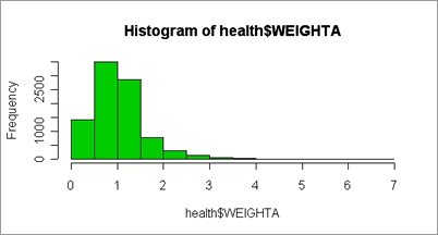
The final weights are a combination of the design weights and the post-stratification weights. The histogram below shows the distribution of the variable WEIGHTA, it is scaled to add (approximately) to the sample size.

Fig 3.3: Histogram of final weights scaled to add to sample size.

A further weight is provided on our data files. This is called GROSSWT and is identical to WEIGHTA except that it has been scaled up to make its total match the mid year population estimate for 16-74 year olds in Scotland. It is required by SPSS in order to get estimates of Design Effects.

The data sets

We have constructed a data set for this analysis with just those variables we will use. The process by which the data set has been constructed and the programmes used to make it from data at Essex data archive) are explained in detail here for anyone who has an interest in this . The identification of the PSUs from the data on the archive required some detective work. It is explained in the comments of the SPSS program used to prepare the data set.

After the PSUs had been identified they were grouped into strata in pairs according to the ranking of their Carstairs index, within regions. Where there were an odd number of PSUs in a region the last stratum was given 3 PSUs.

The information used to derive this information, including the exact Carstairs index values of the PSUs, has been removed from the file to prevent identification.

The variables in the data files are :-