Setting up Model 2 (page 1/5)

Once you have MLwiN installed on the computer that you are using, open MLwiN by locating it in the programmes listed in the windows start menu or by clicking on the MLwiN icon on your desktop.

The default worksheet size for this exercise is 5000 cells which is too small to permit the analysis. However, it is easy to increase the worksheet size.

To do this go to options and make the worksheet 10000 cells (change from 5000). N.B. Do not save worksheet when prompted.

1. No go to the file menu in MLwiN and open lmmd6.ws
2. Choose data manipulation > names.

   

   View the data and notice that the data have been sorted by country code (second column) -all the observations for Austria -the first country in the dataset appear together, then all the observations from the second country and so on.

   N.B. Variables with uppercase names are from aggregate (macro) data. Variables with Lower case names are from the ESS survey (micro).

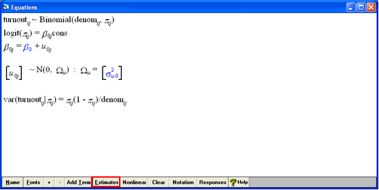
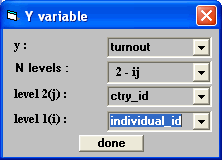
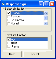
   We have a binary outcome (turnout: 0=didn't vote, 1=voted) so we need to set up a multilevel logistic regression model to model the chance of someone voting. Do this as follows.

3. Go to model equations and you see this



4. Click on the red y variable and choose turnout. We have a 2 level structure with country at level 2 and individual at level 1 specify this structure like this:

   

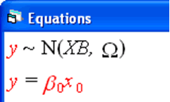
   We need to change the model specification from the basic assumption that y (the dependent variable) is a normally disturbed interval scale variable.

5. Click on the N to change the distribution. Choose binomial logit.

   

   Now the equation looks like this:



6. Click on the red n and choose 'denom'.



7. Click on red x and choose 'cons' and allow this to vary from country to country by clicking the ctry_id box

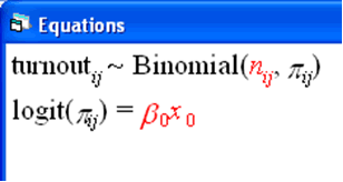
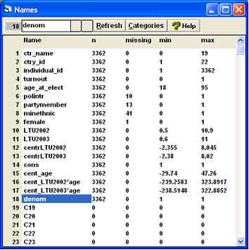
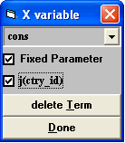
   N.B. 'cons' and 'denom' are two variables that are needed to allow MLwiN to fit a multilevel logistic model. In this example (which is typical of the situation for social science data) both 'cons' and 'denom' are just columns of 1s with the same number of observations as there are individuals in the dataset.

   

   We have now set up Model 2 -the null model

8. It looks like this (click on Estimates button at the bottom of the equations window to see this representation).

As you can see the items in blue are the parameters to be estimated -on the log odds (logit) scale these are the overall mean beta 0 and the between country variance component sigma squared u 0.