C

Ceiling and floor effects

Ceiling effects refer to situations where data points cannot rise above a certain value and floor effects where data points cannot drop below a certain value. This means that the range of values that data can take is restricted.

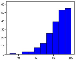
The histogram below exemplifies a ceiling effect. Imagine that it represents a test on which scores can range from 0 to 100. In this case it is apparent that the majority of students achieve the highest possible score, but surely these students are not all at the same level of ability? It may be that the test does not contain enough difficult items and so all those with average or above ability are able to attain the highest score. This histogram resembles half of a normal distribution but this is not always the case with floor/ceiling effects. It is important to watch out for them!

Chi-square

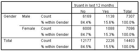
The Chi-square (χ²) test, known in full as the Pearson Chi-square test, is used to check whether two categorical variables are statistically associated by analysising the data in the cells of a crosstabulation (see example of a crosstabulation below). If the chi-square test statistic is significant (i.e. if p < .05) this will suggest there is a significant association between the two variables being explored. See Foundation module 2.2 for an example. the χ² test statistic is also used in logistic and ordinal regression models to asess the improvement in fit or explanatory power of different models.

 

Classification Plot

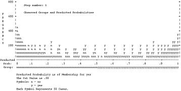
A classification plot is useful in logistic regression for visually exploring how accurately a model predicts a binary outcome by charting both the predicted and actual classifications for the outcome variable. It allows the users to see where misclassifications tend to occur with regard to the probabilities calculated by the model. There is an example of a classification plot below:

Clustering

'Clustering' refers to situations where cases are grouped together in a hierarchical manner. For example, pupils are clustered within classes, classes are clustered within schools, schools are clustered within Local Authorities and so on. Students within the same cluster (the same school, for example) often have a tendency to be more similar to each other than students drawn from different clusters. Clustering can be problematic if not accouted for in the analysis since it can lead to the assumption of Independent Errors being violated. see SLR module 2.6 for more detail.

Confidence interval

When calculating a statistic based on a sample of cases we can not be certain that the value we obtain accurately reflects the value for the entire population. A confidence interval is a range of values (with an upper and lower bound) which we can be confident contains the true value of our statistic. Most confidence intervals are set so that there is a 95% probability that the true statistic is contained within the range, but this can be altered. Confidence intervals are very important for setting bounds on your estimates!

Continuous

Continuous data can be measured on a scale - where data can take a wide range of numeric values and can be subdivided into fine increments. Examples include height and temperature but variables such as test scores can also generate continuous data. Continuous data is referred to as 'scale' in SPSS.

Cooks Distance

Cook's distance is a statistic which provides an indication of how much influence a single case has over a regression model. As a general rule, cases with a Cook's distances of a value greater than one should be investigated further.

Correlation

When two variables have a linear relationship with one another such that one varies systematically with the other they are said to be correlated - they are associated with one another. The strength and direction of a correlation can be represented by a correlation coefficient such as Pearson's r or Spearman's Rho. This coefficient can be used to ascertain how strong the association between variables is and whether it is positive (as one variable increases in value so does the other) or negative (as one variable increases in value the other declines).

Correlation matrix

A correlation matrix is a table that shows all of the relationships between a set of variables (it often also shows whether or not these relationships are statistically significant). There is an example below.

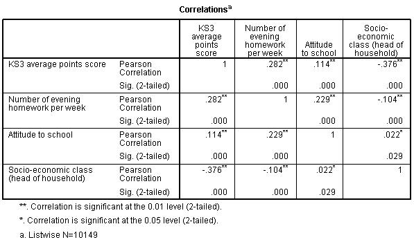
As you can see, sadly this matrix has nothing to do with Keanu Reeves or kung-fu.

Covariance

Covariance is a measure of how much two variables change together. It can be used to calculate Pearson's r. For those of you who want to grasp the concept more mathematically the formula for covariance is:

The difference between each individuals score on variable X and the mean of variable X is multiplied by the difference between their score on variable Y and the mean of variable Y. These 'cross-product deviations' are averaged across the entire sample to provide the covariance. Covariance is therefore the average cross-product deviation.

Cox and Snell R square

This is an adapted version of the R² (coefficient of determination) that can be used in logistic regression. It approximates the proportion of the total variance in the data that the model accounts for (ranging from 0 to 1). It is slightly more basic than Nagelgerke's R² as it is basically calculated by dividing the -2LL of the model by the original -2LL. It can be tested for statistical significance.