|
|
|
|
|
|
|
> 6.0 Introduction>6.1 Imputation or weighting for missing
data?> 6.2 Types of imputation
>6.3 Missing data concepts MCAR, MAR and
MNAR > 6.4 Patterns of
non-response
>6.5 Complicated patterns > 6.6 Software for imputation> 6.7 Features and problems of some software
|
|
|
 top
When a survey has missing values it is often practical to
fill the gaps with an estimate of what the values could be.
The process of filling in the missing values is called
IMPUTATION. Once the data has been imputed the analysts can
just use it as though there was nothing missing.
Imputation is very heavily used for Census data both in
the US and in the UK With census data imputation is used to
fill in data from households and people who failed to
complete a census form (unit non-responders) as well as for
questions people have missed on the form (item non-response).
In 2002 the State of Utah filed a lawsuit against the US
Census bureau claiming the imputation was against the US
constitution (link to details of this). The lawsuit,
which was unsuccessful, was motivated by the state’s
attempt to be assigned a larger population and hence a bigger
share of federal money. The advantage of using imputation for
unit non-response is that all the tables for the census or
survey add up to the same total. This was a major reason for
the use of imputation in the UK 2001 census, known as the One Number Census.
Once you have a data set with
imputed data, it may be tempting to treat it as though it
were real data. For example you might use it to detect
individual influential observations, some of which might be
imputed values. It should not be thought of as real data, but
simply as a convenient way of carrying out statistical
analyses that adjust for the biases due to missing
observations. Diagnostics and data checking should be carried
out on the original data.
|
|
|
|
|
|
|
top
In survey research it is more usual to use weighting
rather than imputation for  unit non
response . Weighting for non-response is covered in
section 5 of the theory part of
this site. But it can become very complicated, especially if
you have a longitudinal survey with several waves. Each
cross-section of the survey can be weighted to make it
representative of all potential respondents at that time.
Alternatively, for a comparison of change over time, the
later wave may be reweighted to match the data collected at
the first wave. This can get complicated, so an imputation
procedure that fills in the missing values for all of the
responses is more practical. Imputation also has the
advantage of being able to handle item non
response as part of the same procedure. unit non
response . Weighting for non-response is covered in
section 5 of the theory part of
this site. But it can become very complicated, especially if
you have a longitudinal survey with several waves. Each
cross-section of the survey can be weighted to make it
representative of all potential respondents at that time.
Alternatively, for a comparison of change over time, the
later wave may be reweighted to match the data collected at
the first wave. This can get complicated, so an imputation
procedure that fills in the missing values for all of the
responses is more practical. Imputation also has the
advantage of being able to handle item non
response as part of the same procedure.
The imputed data can be made available to secondary
analysts and procedures that adjust the standard
errors for the imprecision due to the missing data
are available.
There are currently many new developments in methodology
for handling missing data. We can only cover the bare
essentials here, concentrating on methods that have proved
useful and where software to implement them is easily
available.
A much more detailed description of methods for missing data
(including imputation) is available at the web site developed
by James Carpenter and Mike Kenward http://www.lshtm.ac.uk/msu/missingdata
which, like this site, is sponsored by the ESRC Research
Methods programme. Carpenter and Kenward's site focuses
specifically on missing data for multi-level models, but they
also cover general background concepts.
In their guidelines for handling missing data (click here to read as pdf file)
referring to the choice between weighting and imputation they
state that:
"In practice, multiple imputation is
currently the only practical, generally applicable,
approach (to missing data) for substantial data
sets."
Having struggled to make imputation work correctly for exemplar 6 with various packages, I
am not sure I would agree 100% with its being 'practical,
generally applicable'. Like much applied statistics
imputation seems to be as much an art as a science. I hope
this site may help others in this art.
Gabrielle Durrant is carrying out a review of imputation methods
for the ESRC National Centre for Research Methods.
This deals mainly with single imputations, but covers a much
wider range of new methods than we illustrate here. She has
provided us with a draft of her report.
|
|
|
|
|
|
|
top
There are many different systems of
imputation that may often be used in combinations with one
another. The categories below give general definitions but
some of them can have several different variants.
This is only possible when it may be possible to determine
exactly what the answer to a question should have been from
other sources. For example if a respondent says that they get
a certain benefit, but they don’t know how much it is,
then the survey firm can look it up and complete the data.
This is only possible for a few variables and it can be very
expensive in time and resources.
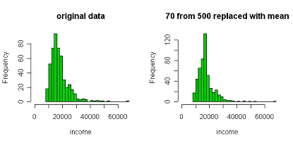
For numerical data the missing values are replaced by the
mean of for all responders to that question or that wave of
the survey. This will get the correct average value but it is
not a good procedure otherwise. It can distort the shape of
distributions and the distort relationships between
variables. The picture below shows what imputing 70 values
out of 500 in a survey of incomes could do to the shape of
the distribution. The mean is the same but everything else is
wrong.
Figure 6.1 Effect of mean imputation on the shape of a
distribution
In hot deck imputation the missing values
are filled in by selecting the values from other records
within the survey data. It gets its name from the way it was
originally carried out when survey data was on cards and the
cards were sorted in order to find similar records to use for
the imputation. The process involves finding other records in
the data set that are similar in other parts of their
responses to the record with the missing value or values.
Often there will be more than one record that could be used
for hot deck imputation and the record that could potentially
be used for filling a cell are known as donor records. Hot
deck imputation often involves taking, not the best match,
but a random choice from a series of good matches and
replacing the missing value or values with one of the records
from the donor set.
Hot deck imputation is very heavily used
with census data. It has the advantage that it can be carried
out as the data are being collected using everything that is
in the data set so far. Hot deck imputation procedures are
usually programmed up in a programming language and generally
done by a survey firm often around the time the data are
being collected. They are very seldom done by secondary
analysts and so we will not be showing examples on the PEAS
web site. The package Stata includes a sophisticated hot deck
procedure written by Mander
and Clayton that can be incorporated into an imputation
procedure. A set of SAS macros to carry out hot-deck
imputation are described in a SAS
technical report contributed by staff members from the US
Census bureau.
Model based imputation involves fitting a statistical
model and replacing the missing value with a value which
relates to the value that the statistical model would have
predicted. In the simplest case we might have one variable
with a missing value which we will call y
which is missing for some observations in the data set. We
would then use the observations in the data set for which
y was measured to develop a regression model
to predict y from other variables. These
other variables have to be available for the cases with
missing values also. We then calculate the predicted value of
y for the missing observations.
One method of
imputing would simply be to replace the missing data with the
predicted values. This has the same disadvantage which we
showed for the mean imputation up above. It tends to give
values that cluster around the fitted prediction equation. A
better procedure is to replace the missing value with a
random draw from distribution predicted for
y. The procedure we have just described
assumes that the regression model is correct and completely
accurate. We only have an estimate of the regression model
not an exact representation of it. So a further step is to
add some additional noise to the imputed value to allow for
the fact that the regression model is fitted with error. When
this is done and all these sources of variability have been
incorporated into the procedure the imputations are said to
be "proper imputation" in that they
incorporate all the variability that affects the imputed
value.
This would be the simplest type of model
based imputation, more complicated methods can be used that
look not only at one variable at a time but model jointly a
whole set of variables. These are discussed in section 6.5 below.
Once data have been imputed one can simply carry on to
analyse the imputed data as if it were the real data. If
there is a substantial amount of missing data the results
that come from this analysis, although on average they will
give good estimates, will be over-optimistic in that they
will be assuming that the missing data really were measured
by the imputed value. We know this is not the case because if
we imputed the same value twice, using methods described
under hot deck or model based imputation, we would not always
get the same imputed values. In hot deck imputation we would
usually get a different choice from potential donor records.
In model based imputation we would select a different value
from the distribution of the predicted values.
In order to incorporate this variation in
the analyses one needs to run the imputation more than once.
This is very straightforward, one simply carries out the
regression more than once and in the first instance looks to
see whether the imputed results are the same for each of the
analyses. They will never be exactly the same and, in order
to incorporate this variation into our estimates of error
there are some relatively straightforward formulae that can
be used. To use the formulae you need to express your results
in terms of statistics that follow a normal or a t
distribution, but this covers a wide range such as means,
proportions and all types of regression.. Ideally, proper
imputation should be used for each of the multiple
imputations.
It is not usually necessary to carry out
the multiple imputation many times, 5 to 10 have been
suggested, but we would suggest rather more (e.g. 20 to 50)
if good estimates of standard errors are required. The
formula for combining imputations works well in practice
since it is usually a much smaller source of error than other
aspects of a survey. More details on multiple imputation can
be found from the relevant part of Carpenter and Kenward's missing data web site
�
|
|
|
|
P|E|A|S project 2004/200
|
|
|
top
These acronyms are used to describe some import and
concepts in missing data analysis that were introduced by
Little and Rubin and are discussed in detail in their classic textbook.
- MCAR is Missing Completely At Random. It means that the
probability of an item being missing is unrelated to any
measured or unmeasured characteristic for that unit. In
survey research this is only likely to apply if data are
missing due to some administrative reason, such as
omissions at data entry.
- MAR stands from Missing At Random. It implies that the
probability of an item being missing depends only on
other items that have been measured for that unit and no
additional information as to the probability of being
missing would be obtained from the unmeasured values of
the missing items. This is the assumption underlying most
imputation methods, since they use the observed data to
predict what is missing.
- MNAR stands for Missing Not At Random and it implies
that the missing observations would, if measured, have a
different distribution from that predicted from what is
observed. For example, those refusing to answer income
questions might have a different distribution of incomes
compared to other people with similar answers to other
questions who did answer the income questions. It is not
possible to correct data for a MNAR mechanism, except by
using outside information. Sensitivity analyses to
different degrees of MNAR is another possible
approach.
|
|
|
|
|
|
|
top
Although the basic ideas of imputation are simple, the
practicalities are
very complicated. Things are very much easier if the pattern
of non-response is nested. By nested we mean that variables
can be ordered in such a way that once a case has a missing
value on one observation it is then subsequently missing on
everything else. This sort of pattern is fairly common when
we have a longitudinal study and data are missing simple
because people drop out of the study. In most other cases the
missing values do not have a nested pattern.
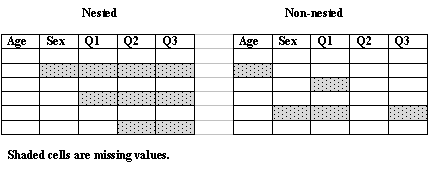
It is very much more straight forward to carry out
imputation for a nested pattern of non-response’ In
the example above imputation would proceed by first imputing
sex from age, then Q1 from age and sex, then Q2 from age, sex
and Q1, and Q3 from age, sex, Q1 and Q2. So only a series of
four simple imputations are required. For the later
regressions, for example when predicting Q1 from age and sex,
the imputed values are used in the regression, and one ends
up with a complete set of data. In the non-nested case this
is considerably more difficult and special procedures are
required for analysing the data. Often data are approximately
nested and this can be very helpful in running these
procedures.
The first stage in any missing data analysis, is to
investigate the pattern of non-response to find out which
values are missing and in what combinations. This also allows
the user to understand the structure of the data and to know
which variables have the most missing data.
|
|
|
|
|
|
|
top
There is no uniform solution on how to handle complicated
missing value
patterns, and they all involve making some strong assumptions
about the model that has generated the data. But when data
are missing on several variables it is important to use some
procedure that imputes them all together, rather than one
variable at a time. This ensures that the imputed data are
related to each other (e.g. have similar correlations) in the
same way as those data that are observed. Several approaches
have become available for practical use in recent years.
Some algorithms start by approximating the pattern of
non-response to a nested pattern. The procedure starts by
predicting the missing values for the variable with the
fewest missing values from variables with complete data.
Then the complete and imputed are used to predict the
missing values for the next variable, and so on until all
the missing data are replaced. A problem with this method
is that variables that have their data replaced first use
reduced models and may have missed some important
dependencies.
To overcome this problem the whole cycle of predictions
for each variable is repeated using data imputed at the
first stage. At each stage variables that were missing are
predicted from all of the imputed data from the other
variables. The repetitions carry on until the procedure is
stable. This process is called multiple imputation with
chained equations. A model suitable for each variable is
selected. A binary variable is predicted from a logistic
regression, a continuous variable from an appropriate
regression, and so on. The user must specify the models
for each variable.
Once the predicted values are obtained the imputed
values are randomly sampled from the predictive
distribution for the missing data. This is usually carried
out with proper
imputations and multiple
imputations> can be obtained. Several research
groups have provided resources that implement these methods
in different packages and their web sites provide links to
helpful examples and explanations.
These methods can have some practical problems. Details
are given in the section on software
below and the specific features of different
implementations are discussed in section 6.7.1. Some statisticians also
query them on the theoretical grounds that the joint
distribution, implied by the procedure, may not exist.
Various versions of these techniques are available, as
detailed in the section on software (Section
6.6 below). Some of these allow the links in the chain
to take different types, such as a hot-deck steps. We will
use the term 'chained methods' to refer to this general
class of methods. that cycle round each variable in turn.
Individual links in the chain are most commonly regression
prediction, but other methods such as mean imputation or
hot deck steps could also form links.
Another method that is used is to model the data as a
sample from a joint distribution. The most common choice is
a multivariate normal distribution. The theory behind this
is described in Jo Schafer's excellent monograph on missing data.
It might seem surprising that something like a 1/0 variable
could be approximated by a normal variable but practical
experience suggests that this procedure works reasonably
well in many cases. In this case the imputed values need
to be forced to 1/0 values, either during or after the
imputations, using some rule, such as the value closest to
the imputed value.
The first step in these procedures is to estimate the
parameters of the multivariate normal distribution, making
use of all the available data including those partially
observed. An iterative method known as the EM algorithm is
used for this. This gives expected mean values for the
missing data. . The next step samples from the predictive
distribution of the missing data and incorporates
uncertainty in the fitted values, making this a proper
imputation. Finally several multiple
imputations are generated. . The support pages of
the SAS web site provide a useful
overview of this method and basic references.
Schafer has also developed theory and models for binary
and general categorical data (CAT) and for combinations of
binary and normal data as well as longitudinal or panel
data (PAN). Some software is available and details are
given in Schafer's
textbook. But these have not been much taken up by
statistical practitioners. This may be due to their
computational demands for any but the smallest models and
other practical problems with implementing them.
|
|
|
|
P|E|A|S project 2004/2005/2006
|
|
|
top
Simple imputation methods (one variable at a time) can
readily be programmed using commands such as regression
analyses in standard packages.
Multiple
imputation procedures suitable for complex surveys,
discussed in section 6.6 , are more
challenging. These are most commonly available as part of
contributed packages or add-ons.
After a multiple imputation procedure has been carried out
the user has a new data file or files that give several
copies of the complete data. Often this will be a file in
which the imputed data sets are stacked one above the other,
indexed by the number of the imputation. Post-imputation
procedures involve analysing each of the imputed data sets
separately and averaging the results. The differences between
results obtained on the different data sets can be used to
adjust the standard
errors from statistical procedures. This process has
been automated in some packages, so that one command will
produce the averaged analyses and the results with adjusted
standard errors.
This process works well for procedures such as regression
analyses. For simple exploratory analyses it may be
sufficient to work with a single data set, unless there is a
substantial proportion of missing data for one or more of the
variables being analysed. One way to check this is to run the
exploratory procedures on different imputations to get an
informal estimate of the variation between the
imputations.
Table 6.1 summarises some of the procedures available for
handling missing data in the packages featured on this
site.
| � |
SAS
|
SPSS
|
Stata
|
R
|
| missing value patterns |
MI |
MVA |
nmissing
(dm67)
mvmissing(dm91)
|
md.pattern(mice)
prelim.norm(norm)
|
| repeated measures analysis |
MIXED not GLM (*) |
� |
? |
pan |
| single imputation |
� |
MVA |
impute
uvis(ice)
|
em.norm
da.norm
|
| multiple imputation |
MI
IMPUTE (IVEWARE)
|
MVA with EM algorithm |
ice (ice) |
norm (norm)
mice (mice)
|
| post-imputation |
MIANALYZE |
� |
micombine
(r-buddy.gif" alt='warn')
mifit and others (st0042)
|
glm.mids,pool(mice)
mi.inference(norm)
|
(* PROC GLM in SAS does
listwise deletion and so does not allow for missing values.
This is also true of SPSS repeated measures analyses)
Items in
(brackets) indicate that the item is a set
of contributed procedures. In particular the following
research groups have provided routines and their web sites
are helpful.
- IVEWARE software for SAS developed by
a group at the University of Michigan.This is a set of
SAS macros runs a chained equation analysis in SAS. It
can also be run as a stand-alone package.
- The MICE library of functions for Splus/R
has been written by a group at the University of Leiden
to implement chained methods.
- Chained equations have been implemented in Stata by
Patrick r-buddy.gif" alt='warn' of the MRC Clinical
Trials Unit in London. The original procedure was called
mvis and is described in the Stata journal (Royston,
P. 2004. Multiple imputation of missing values. Stata Journal 4: 227-241.). A
more recent version called ice is now available (
Royston, P. (2005), Multiple imputation of missing
values: update, Stata Journal 5, 188-201). Both
can be dowloaded from the Stata journal by searching net
resources for mvis and for
ice respectively.
- Methods based on the multivariate normal distribution
have been developed by Jo Schafer of Penn State University
using his program NORM can be run as a stand alone
resource and is implemented in SAS and in R/Splus. There
appear to be problems with the current implementation in
R that are being taken up with the authors.
The SPSS Missing Value
Analysis (MVA) software has been criticised in an article in
the American Statistician von Hippel P, Volume 58(2),160-164. The
MVA procedure provides two options. The first is a
regression method that uses only the observed data in the
imputations and the second is based on the normal
distribution and resembles the first step of the NORM
package. Neither are proper imputations.
Other specialised software for imputation, such as SOLAS, has
to be purchased separately and are not featured on the PEAS
site. SOLAS links to SPSS and implements various methods,
including imputation using a nested procedure. The SOLAS
web site has useful advice on imputation practicalities,
and it has now been extended to cover multiple imputation procedures.
The programs MLWin and
BUGS can be used for imputation. Carpenter and Kenward's
missing data site has details.
Despite having been written a few year's
ago, an article by Horton and Lipsitz (Multiple
imputation in practice: comparison of software packages for
regression models with missing variables. The American
Statistician 2001;55(3):244-254.) that can be accessed
on the web, has lots of useful practical advice
on imputation software.
The programs that implement these methods are fairly new
and several of them are still under development. They have
all been written in response to user needs and have many
helpful practical features. In the next section we will
mention some of the good features that exist in some
implementations, and also some caveats.
Things can easily go seriously wrong and you should always
check that the data are reasonable. Unbounded imputation from
a normal distribution can sometimes give extremely high
values that affect the mean. A minimum is to look at some
histograms of the observed and imputed values.
Details that ensure that the imputed values make sense
need to be considered when an imputation scheme is designed.
For example, if one imputes missing values for the two
questions "do you smoke cigarettes?" and "how many cigarettes
do you smoke?" we need to be careful that numbers of
cigarettes are not imputed for non-smokers.
Imputed values also need to be plausible. If a variable
for number of visits to the doctor is being imputed it needs
to have integer values. A predicted value may also sometimes
be outside the range of reasonable values. Various methods,
such as rounding after the imputations and setting limits can
be used to overcome these difficulties. This process has been
criticised as introducing biases, and it has ben suggested
that the unrounded data should be retained to avoid this. For
practical survey work it is difficult to envisage not doing
something to fix the data.
A general approach, sometimes called 'predictive matching',
matches the predictive value to the prediction for an
observed case and uses the true value of the case for
prediction.. This might appear to solve a lot of problems at
once, but it is not well understood and recent work suggests
that it may sometimes do some very odd things.. We would not
advise its use.
|
|
Note that there are currently problems with both
MICE and NORM for R. We
will update the site when these are resolved.
Also a new version of mice (renamed ice) is soon to
be available for Stata.
|
|
P|E|A|S project 2004/2005/2006
|
|
|
top
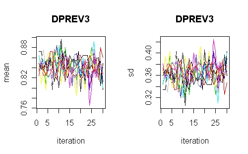
Most multiple
imputation procedures involve iterative schemes
either to get the parameters or to cycle round the variables.
Some programs provide software to check this. The R
implementation of chained equations does this as does the
SAS implementation of NORM (PROC MI). This illustration is
from R and shows a well converged iterative scheme. If these
plots have the iterations separated, or have obvious trends
then something is wrong or perhaps the iterations need to be
run for longer.
Chained equation procedures will converge better if they
have good starting values. Some programs fill in the missing
values at random (R MICE and Stata's old versions). The
IVEWARE procedures in SAS and the new Stata version uses a
sequence of regression models built up from an approximation
to a nested pattern. This is
important when there are some strong relationships between
variables in a data set that might otherwise take a long time
to come right.
The R version of NORM is
currently not functioning properly on large data sets (July
05). The current R implantation (2.01) does not have the MICE
package as an option and contact with the authors suggest a
problem with resources to support it (July 05). Further
information about solutions to these problems will be added
when they are resolved.
All of the imputation are computer intensive and some of
the models fitted here took hours to run.
Fitting or computing problems can invalidate imputation
results. This happened in one way or another with each of the
packages. The programs will often warn and/or stop with an
error when things are going wrong. The Stata chained equation
package (mvis, now ice) trapped  almost all
errors. But, in other cases, the imputed data may be
generated but, on inspection, are clearly inadequate.
Examples include almost all
errors. But, in other cases, the imputed data may be
generated but, on inspection, are clearly inadequate.
Examples include
- very large, near infinite values for some continuous
variables
- categorical variables where all of the missing data
goes into one category
- imputations where the imputed value of some
observations is the same for every imputation
- too many missing values for the available data and the
model being fitted
It is hard to give precise rules for when this might
happen, but several things seem to make it more likely
- having a lot of categorical variables with many
categories so that the cells formed by them are
sparse
- having some very strongly associated variables
- fitting very large and/or complicated models, although
this is often recommended by imputation experts
We strongly recommend that you spend
time checking for this kind of error whenever you carry out
an imputation procedure. Just eyeballing the raw
data and doing simple tables is as good as any fancy
methods.
The SAS and Stata implementations of offer the option of
predictive matching, as described in Rubin's textbook (see list of texts).
Experimenting with this option has revealed problems with the
method. Communication with the author of the Stata code
(Patrick Royston) revealed that he had problems with it too
and the revised version of his Stata routine
(ice) does not set it as a default method.
We suggest that you take care when using this method and pay
special attention to diagnostics and to checking
convergence.
The SAS PROC MI allows the option of rounding data during
the imputation process when this is a feature of the data.
This sounds like a good idea. But when we tried it on
exemplar 6 we found it introduced a bias when used with
binary data, compared to a logistic model. We suggest that it
would be better to impose the restrictions after the data are
imputed.
All of the chained equation methods allow continuous and
categorical variables to be modelled. In addition, IVEWARE
allows count data to be modelled as a Poisson variable and a
mixed variable type with a proportion of zero values. The
Stata implementation of chained equations (mvis/ice) allows
ordered logistic regression, which is useful for many survey
questions. The packages all allow individual selection of
models for each variable, though this would be tiresome for a
big survey.
Other features can also be very helpful. IVEWARE has
several of these It allows bounds to be set within the
imputation steps, and these bounds can be functions of other
variables. It also allows a stepwise procedure that will
select a subset of the variables automatically, which can
speed convergence time. Interactions can be included in the
fitted model.
The new version of chained equations (ice) for Stata
incorporates several useful new features. Its new features
allow fuller model specification with individual prediction
equations. It also allows interactions to be fitted and dummy
variables to be generated from factors to use in other
equations.
Post-imputation procedures often need to be run in two
stages and the results don't have a very user-friendly
layout. The exception is micombine in Stata
which is easy to use and produces nice output. The SAS PROC
MIANALYZE procedure is awkward to use, but once it has worked
its output is very helpful and can be used to guide how many
imputations should be run in future.
|
|
|
|
P|E|A|S project 2004/2005/2006
|
|