|
|
|
| |
|
|
| |
>> 4.1 Background >>4.2 Sample
design >>4.3 Features of this exemplar
>> 4.4
Getting started
|
|
|
 top
This exemplar is based on data from WERS98 to look at the relationship
between workplace composition and equal opportunities policies.
The example was motivated by analysis reported in the Department
of Trade and Industry (DTI) report ‘Equal
Opportunities policies and practices at the workplace: secondary
analysis of WERS98. Anderson, T., Millward, N., and Forth,
J. DTI Employment Relations Research Series No. 30).
The exemplar aims to illustrate analysis of survey data where a key feature
of the design is that the sampling fractions (and hence the survey weights)
are very different across strata.
The data for this exemplar were obtained from the ESRC data archive,
but they have been altered to prevent the disclosure of individual
workplaces using the principles described here. The way in which
the data provided here relates to the data from the archive can
be viewed here.
|
|
|
|
|
|
|
top
WERS98 is a survey of workplaces in GB with 10 or
more employees, the sample being selected from the ONS’s Inter-Departmental
Business Register (IDBR). Background data and reports on WERS can be
found here.
The WERS data
dissemination service provides links to a number of very helpful
reports and explanatory papers about technical aspects of the survey
design and how to analyse it..
The size distribution of workplaces in the GB is extremely skewed, with,
at one end of the spectrum, 58% of workplaces having between 10 and 24 employees,
but just 1% of workplaces having 500 or more employees. For any moderately
sized sample, an equal probability sample design would give extremely small
numbers of larger workplaces. So, to allow for separate analysis by size,
the sample for WERS98 was selected so as to give a reasonably large sample
size per size-band. This was achieved by systematically increasing the sampling
fraction as the size of workplace increased. The table below gives the numbers.
|
no of employees at workplace
|
population of workplaces
|
sample of workplaces selected
|
sampling fraction
|
|
10-24
|
197,358
|
362
|
1 in 545
|
|
25-49
|
76,087
|
603
|
1 in 126
|
|
50-99
|
36,004
|
566
|
1 in 64
|
|
100-199
|
18,701
|
562
|
1 in 33
|
|
200-499
|
9,832
|
626
|
1 in 16
|
|
500+
|
3,249
|
473
|
1 in 17
|
|
TOTAL
|
341,411
|
3192
|
-
|
Table 4.1: WERS Sampling fractions
In addition the sample was stratified by the Standard Industrial
Classification (SIC), although within size-bands, the sampling fraction by
SIC group was kept roughly constant. WERS98 can be thought of as an extreme example of a sample design using
stratification with unequal probabilities of selection. The strata
are ‘size by SIC’ categories.
To derive unbiased estimates for workplaces the very large mismatch between the sample distribution and the population distribution has to be addressed. This is achieved by weighting the sample data, the weights being calculated as the inverse of the probability of selection.
WERS98 also included a sample of employees but we have not made use of
that dataset here.
|
|
|
|
|
|
|
top
|
what is this?
|
details for this survey
|
| Disporportionate stratification |
|
|
Effects of weighting on  standard errors standard errors
|
|
|
| Logistic regression for survey data |
|
|
| Strata with large sampling fractions so
that a finite population correction may be needed
|
|
|
Table 4.2: Features of this exemplar
|
|
|
|
|
|
|
top
|
From links in this section you can:-
- Downlaod or open the data files
- Analyze them with any of the 4 packages you have available
- View the code (with comments) and the ouput, even if you
don't have the software.
To start, click the mini guide for the statistical package
you want to use to analyse Exemplar 4.
For additional help click on the appropriate novice guide.
For details of the data set see below.
|
|
|
|
| |
|
|
|
|
|
|
|
Table 4.3: Data sets and code
|
* SAVE these files to your computer
The html files are provided so you can view the code
and the output without having to run the programs.
|
|
|
|
|
|
|
|
|
top
The analysis carried out here demonstrates the impact that
survey weights can have on survey estimates and their standard errors.
The example looks at the proportion of workplaces that have an equal opportunities
policy, and the relationship between this proportion and other workplace
characteristics, in particular the percentage of employees that are female,
disabled, or from a minority ethnic group.
| Weighting |
proportion with eo policy
|
standard error |
|
unweighted
|
81.1%
|
0.81%
|
|
weighted
|
67.3%
|
1.81%
|
|
base=2 191 workplaces
|
Table
4.3: Effect of weights on % workplaces with equal opportunites policy
We can see that adding the survey weights greatly reduces
the estimate of the percentage of the workplace with an equal opportunities
policy. This happens because there is a very wide range of weights (see below). Also the weighting ‘weights down’ large
workplaces and ‘weights up’ smaller workplaces, and having
an equal opportunities policy is very strongly related to workplace size.
The standard error
is more than doubled in the weighted analysis. We can see in Table 4.4 that the largest workplaces nearly
all have an equal oportunities policy. For this outcome the optimum weighting strategy would have been to
'weight down' these strata because they are very homogeneous. But the opposite is true for the design of this survey. Of course this conclusion only applies
to this outcome. See the theory section for a discussion of this.
| number of
employees
|
Proportion of workplaces with an equal
opportunites policy (weighted estimate)
|
| 10-24 |
0.63 |
| 25-29 |
0.65 |
| 50-99 |
0.72 |
| 100-199 |
0.81 |
| 200-499 |
0.87 |
| 500+ |
0.91 |
Table 4.4: Proportions of workplaces with an equal opportunities policy by number of employees
Both the standard errors shown in Table 4.3 allow for the stratification. An unweighted mean with no stratification would have had a standard error
of 2.01%, showing that there has been a small gain in precision from the stratification.
|
|
|
|
|
|
|
top
We now compare other workplace characteristics,
such as the percentage of employees that are female, disabled, or from a minority
ethnic groups between workplaces with and without an equal opportunities (eo) policy. We start with bivariate analyses, that simply check whether
the percentage of employees in each of these groups differs by whether or
not there is an equal opportunities policy. The unweighted and weighted results are shown in the table below.
| |
type of estimate
|
'eo' workplaces
|
'non eo' workplaces
|
difference 'eo' minus 'non eo'
|
standard error of difference
|
|
mean percentage
female
|
unweighted
weighted
|
40.8
59.6
|
51.8
42.7
|
10.8
16.9
|
1.6
2.9
|
|
mean percentage from
minority ethnic groups
|
unweighted
weighted
|
5.6
5.8
|
3.8
3.3
|
1.8
2.7
|
0.6
0.7
|
| percentages
no disabled employees
some but fewer than 3%
more than 3%
|
unweighted |
53.1
38.8
8.0
|
69.2
22.5
8.1
|
-16.1
16.2
-0.1
|
2.8
2.7
1.5
|
percentages
no disabled employees
some but fewer than 3%
more than 3%
|
weighted |
77.5
12.9
9.6
|
81.8
8.0
10.2
|
-4.3
4.9
-0.5
|
3.5
1.7
3.1
|
Table 4.5: Comparison of other variables between workplaces 'eo' and no 'eo' policy.
We see from this that the survey weights have rather a large
impact on the differences in means. Most strikingly, without weights the mean
difference in the percentage of women between workplaces with and without
an equal opportunities policy is just 11%. But with weights the difference
is 17%. It is also striking that adding the weights also increases
the standard errors of the differences quite considerably.
We can also see that the unweighted analysis suggests that there are differences
between 'eo' and 'no-eo' workplaces in the percentage of disabled
empoyees. But the weighted anlysis, adjusting for the survey design
does not confirm this. This difference was also seen when a chi-squared
test was used. The unweighted chi-squared test gave a p-value
of 0.000000005 for the association between 'eo'
and the grouped variable for disabled employees. Whereas the weighted
chi square test, adjusted for the design (theory
link ) gives a p-value of 0.20 (not significant).
The natural next step is to include the three employee characteristic
variables in a single regression model, with ‘equal opportunity policy’
as the dependent variable. This suggests a logistic regression model. Again
we compare unweighted and weighted model coefficients to check for the impact
of the weights.
|
|
|
|
|
|
|
top
The table below gives two different logistic regressions to predict the log-odds of having an equal
opportunities policy. The first is unweighted and makes no use of the survey design. The second is a weighted analysis
and adjusts for the survey design.
|
independent variables
|
logistic regression coeffecient (log odds)
|
| |
unweighted estimates
(standard error)
|
weighted estimate (standard
error)
|
|
percentage female
|
0.0140 (0.003)****
|
0.0190 (0.003)****
|
|
percentage from minority ethnic groups
|
0.017 (0.007)*
|
0.028 (0.011)*
|
disabled employees
no disabled employees
some but fewer than 3%
more than 3%
|
reference category
0.85 (0.13)***
0.11 (0.21)
|
reference category
0.68 (0.21)**
-0.19 (0.27)
|
|
**** = p < 0.0001 *** = p< 0.001 **=p<0.01 *=p<0.05
|
Table 4.7: Logistic regression for predicting 'eo' workplaces.
Comparing the two columns from this table we see, again,
that the survey weights has changed the estimate. The coefficient for the group 'more than 3% disabled', which changes from positive to negative after weighting the data.
But neither coefficient is significantly different to zero, so this is probably
less important than the fact that the weighted estimates for ‘female’
and ‘minority ethnic’ increase by about 50% after applying the
weights.
Note again that the standard errors are larger for the weighted than for
the unweighted estimates.
The reason the weights have such a large impact on the survey estimates for WERS98 is that
the weights adjust for the very large skew in the sample towards larger workplaces. In other words, the weights give greater ‘weight’ to smaller establishments that are under-represented in the survey. A natural question that arises from this is, if we control for workplace size in the regression models, will the weights still make a difference. And,
if weights no longer make a difference, is it legitimate to use unweighted data and to profit from the smaller standard errors?
To test this we can run the same logistic regression model as we did above but now adding a ‘workplace size’ provided as a set of six groups as an extra predictor. This gives the following co-efficients.
|
independent variables
|
logistic regression coeffecient (log odds)
|
| |
unweighted estimates
(standard error)
|
weighted estimate (standard
error)
|
|
percentage female
|
0.017 (0.02)****
|
0.020 (0.003)****
|
|
percentage from minority ethnic groups
|
0.016 (0.007)*
|
0.029 (0.012)*
|
disabled employees
no disabled employees
some but fewer than 3%
more than 3%
|
reference category
0.18 (0.16)
0.00 (0.22)
|
reference category
0.68 (0.21)***
-0.22 (0.37)
|
|
**** = p < 0.0001 *** = p< 0.001 **=p<0.01 *=p<0.05
|
Table 4.8: Logistic regression for predicting 'eo' workplaces adjusted for workplace size in 6 categories.
Comparing the two columns from this table we see, again,
that weighting has changed the estimates. The coefficient for the group 'more than 3% disabled', which changes from positive to negative after weighting the data.
But neither coefficient is significantly different to zero, so this is probably
less important than the fact that the weighted estimates for ‘female’
and ‘minority ethnic’ increase substantially after applying the
weights. Notice also the larger standard errors associated with the weighted estimates.
This may appear to contradict the comments on the effect
of weighting on regressions (theory section section 4.8). In this section we claimed
that weighting should not be necessary if a model was fully specified, so
that the residuals no longer correlated with the weights. Here we have included
the major factor affecting the weights (size of workplace) in the model. So
we might expect that this would make the residuals uncorrelated with size
of workplace, and hence with the weights. There are two reasons why this conclusion
might not follow here:-
- Our measure of workplace size is not identical to that used in the design. Some workplaces were found to
have a different number of employees than was recorded on the sampling frame. Also, to protect the
identity of respondents, our data set does not differntiate between the largest sub-groups used in the startification.
- We are fitting a non-linear logistic model.
The second of these is probably the more important here.
The model is very highly non-linear, as we illustrate in Figure 1. This shows the fitted values for a further model that dropped out the disabled variable and fitted the percentage of female employees as a category.
The figure shows the fitted values by workplace size for workplaces with different proportions of female employees. We can see that there are substantial differences between the effects of the gender of the workforce between the weighted and unweighted analysis. There are
several places with fitted values close to 100% where the residuals are not
symmetric. The guideline about a fully specified model only applies when the
model is a correctly specified linear model.
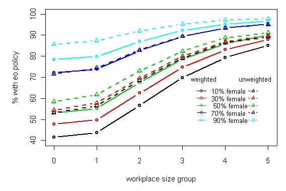 Figure 1: Model fitted values
by workplace size group and percentage female. Fitted values are
shown for ethnic group employees fixed at 2%.
|
|
|
|
|
|
|
top
In the analyses presented above we have been ignoring the
finite population correction (FPC) (see theory section 8.1). The sampling
fraction in some of the strata in this survey is quite large. The highest
sampling fraction is 58% . So if we want to make inferences for the
workplaces existing in the UK in 1998, we should consider the effect of calculating
standard errors with allowance for the FPC.
An example of this might be the calculation of the percentage
of workplaces with an equal opportunities policy. We might wish to estimate
this in order to know how many firms might need to be targeted in order to
improve this situation. Applying the FPC to these
estimates we obtain the figures below for the estimates and their standard
errors.
|
workplace size
|
proportion
|
average FPC
|
standard error (no FPC)
|
standard error (with FPC)
|
| All |
67.53
|
0.056
|
1.810
|
1.810
|
| 10-24 |
63.43
|
0.014
|
3.28
|
3.28
|
| 25-49 |
64.80
|
0.014
|
3.49
|
3.48
|
| 50-99 |
71.87
|
0.029
|
2.64
|
2.62
|
| 100-199 |
81.25
|
0.049
|
2.35
|
2.33
|
| 200-499 |
86.79
|
0.087
|
2.04
|
2.01
|
| 500+ |
91.29
|
0.147
|
1.83
|
1.76
|
Table 4.9: Effect of FPC on standard errors
We can see from the table above that the FPC makes very
little difference to the standard errors. As expected the effect is greatest
in the large workplaces that are more likely to be in the strata with the
larger sampling fractions (see theory section 9.3). But even in these
strata the effect is very small.
The design effects calculated by Stata for this exemplar (see Stata output
last analyses carried out) illustrate the different
ways that a design effect can be calculated for subgroups. This is discussed in the theory section on subgroups.
|
|
|
|
|
|
|
top
|
Technique
|
SAS
|
Stata
|
R
|
SPSS Survey
|
|
Unvariate
tables with
standard errors for % in
each category
|
yes
|
yes
|
yes
|
yes
|
|
Tables
with adjusted chi squared tests
|
not in version 8
|
yes
|
yes- but limited and output
needs a lot of work
|
|
|
Logistic regression
for survey data
|
version 9
|
yes
|
yes
|
version 13
|
|
|
|
|
|
|
|
top
This was a survey of workplaces taken from a business register. Thus there was no
clustering by the addresses
of the workplaces. The whole survey incorporated a cross-sectional survey of
employees, a longitudinal survey and a survey of the employees within the workplaces.
A
technical report describes the design in detail.
The sample was selected from strata formed by classifying workplaces by industry and by the estimated numbers in the workforce (as recorded on the business register). When the final sample was asembled a few strata had obtained results from only one workplace. This could have caused problems at analysis and so these were polled with other similar strata. This
resulted in 71 strata .
The major factor that determined the weights was the different
sampling fractions used for different sizes of workplace.
Some further weighting was used to allow for deficiencies in the sampling
frame that were discovered during the field work. Some large weights were
capped using a complicated procedure and the final weights were rescaled to
add to the sample size (2,191). A grossing up weight is
also supplied with the survey data which adds to the total workplaces in the UK (over 250 thousand). Figure 4.2 illustrates the range of these grossing up weights and the very small weights assigned to large workplaces relative to small ones.
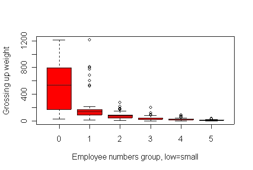
Figure 4. Boxplot of weights exemplar 4
|
|
|
|
|
|
|
top
| Variable |
Label |
|
est_wt
|
survey weight |
|
grosswt
|
grossing up weight |
|
strata
|
stratification variable |
|
eo
|
equal opportunites policy 1=yes 0=no (recoded from IPOLICY) |
|
female
|
percentage of employees at workplace female |
|
disabgp
|
0 = no disabled employees 1=some but fewer than 3% 2= 3% or more disabled |
|
serno
|
serial number (scrambled) |
|
ethnic
|
percentage of employees at workplace from minority
ethnic groups
|
|
nempsize
|
workplace size 0=10-24 1= 25-49 2=50-99 3=100-199 4=200-499 5=500+ |
|
sampfrac
|
sampling fraction in each stratum |
peas
project 2004/2005/2006
|
|
|
|
|
|
